使用 Tidyverse
Tidyverse 是資料科學家在日常資料分析中常用的 R 套件集合。 其包含資料匯入的套件 (readr)、資料視覺效果 (ggplot2)、資料操作 (dplyr、tidyr)、功能性程式設計 (purrr) 和模型建置 (tidymodels) 等。tidyverse 中的套件旨在無縫地協同運作,並遵循一組一致的設計準則。
Microsoft Fabric 會以每個執行階段版本,來散發最新的 tidyverse 穩定版本。 匯入並開始使用您熟悉的 R 套件。
必要條件
取得 Microsoft Fabric 訂用帳戶。 或註冊免費的 Microsoft Fabric 試用版。
登入 Microsoft Fabric。
使用首頁左下方的體驗切換器,切換至 Fabric。
![體驗切換器功能表的螢幕擷取畫面,顯示選取 [資料科學] 的位置。](media/tutorial-data-science-prepare-system/switch-to-data-science.png)
開啟或建立筆記本。 若要了解操作說明,請參閱如何使用 Microsoft Fabric 筆記本。
將語言選項設定為 SparkR (R),以變更主要語言。
將筆記本連結至 Lakehouse。 在左側選取 [新增] 以新增現有的 Lakehouse 或建立 Lakehouse。
載入 tidyverse
# load tidyverse
library(tidyverse)
資料匯入
readr 是一個可提供讀取矩形資料檔案工具的 R 套件,例如 CSV、TSV 和固定寬度檔案。
readr 提供快速且易記的方式來讀取矩形資料檔案,例如提供函數 read_csv() 和 read_tsv(),用於分別讀取 CSV 和 TSV 檔案。
我們先建立 R data.frame,使用 readr::write_csv() 將其寫入 Lakehouse,並使用 readr::read_csv() 讀回。
注意
若要使用 readr 存取 Lakehouse 檔案,您需要使用檔案 API 路徑。 在 Lakehouse 總管中,以滑鼠右鍵按一下您想要存取的檔案或資料夾,並從內容相關的功能表中複製其檔案 API 路徑。
# create an R data frame
set.seed(1)
stocks <- data.frame(
   time = as.Date('2009-01-01') + 0:9,
   X = rnorm(10, 20, 1),
   Y = rnorm(10, 20, 2),
   Z = rnorm(10, 20, 4)
 )
stocks
然後,我們使用檔案 API 路徑,將資料寫入 Lakehouse。
# write data to lakehouse using the File API path
temp_csv_api <- "/lakehouse/default/Files/stocks.csv"
readr::write_csv(stocks,temp_csv_api)
從 Lakehouse 讀取資料。
# read data from lakehouse using the File API path
stocks_readr <- readr::read_csv(temp_csv_api)

# show the content of the R date.frame
head(stocks_readr)
資料整理
tidyr 是一個可提供處理雜亂資料工具的 R 套件。
tidyr 中的主要函數旨在協助您將資料重塑為整潔的格式。 整潔的資料具有特定的結構,其中每個變數都是一個資料欄,而每個觀察都是一個資料列,這可讓您更輕鬆地在 R 和其他工具中使用資料。
例如,gather() 中的 tidyr 函數可用於將寬資料轉換為長資料。 以下列出了範例:
# convert the stock data into longer data
library(tidyr)
stocksL <- gather(data = stocks, key = stock, value = price, X, Y, Z)
stocksL
函數程式設計
purrr 是一個可提供完整且一致工具集來處理函數和向量的 R 套件,藉此增強 R 的功能性程式設計工具組。 開始使用 purrr 的最佳起點是 map() 函數系列,這可讓您以更簡潔且更便於閱讀的程式碼來取代許多迴圈。 以下是使用 map() 將函數套用至清單各元素的範例:
# double the stock values using purrr
library(purrr)
stocks_double = map(stocks %>% select_if(is.numeric), ~.x*2)
stocks_double
資料操作
dplyr 是一個可提供一致動詞集的 R 套件,可協助您解決最常見的資料操作問題,例如根據名稱選取變數、根據值挑選案例、將多個值減少至單一摘要,以及變更資料列的順序等。以下是部分範例:
#  pick variables based on their names using select()
stocks_value <- stocks %>% select(X:Z)
stocks_value
# pick cases based on their values using filter()
filter(stocks_value, X >20)
# add new variables that are functions of existing variables using mutate()
library(lubridate)

stocks_wday <- stocks %>%
    select(time:Z) %>%
    mutate(
        weekday = wday(time)
    )

stocks_wday
# change the ordering of the rows using arrange()
arrange(stocks_wday, weekday)
# reduce multiple values down to a single summary using summarise()
stocks_wday %>%
    group_by(weekday) %>%
    summarize(meanX = mean(X), n= n())
資料視覺效果
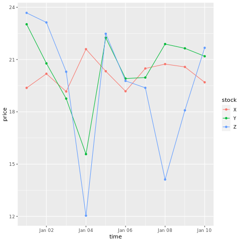
ggplot2 是一個根據圖形文法,以宣告方式建立圖形的 R 套件。 您將提供資料,說明 ggplot2 如何將變數對應至美學、要使用哪些圖形基元,並且會處理詳細資料。 以下列出了部分範例:
# draw a chart with points and lines all in one

ggplot(stocksL, aes(x=time, y=price, colour = stock)) +
  geom_point()+
  geom_line()
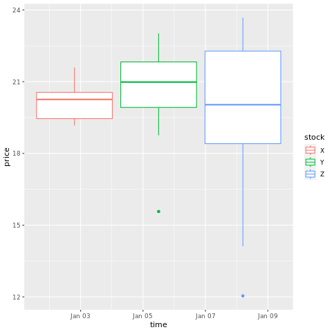
# draw a boxplot

ggplot(stocksL, aes(x=time, y=price, colour = stock)) +
  geom_boxplot()
模型建置
此 tidymodels 架構是使用 tidyverse 準則建立模型和機器學習的套件集合。 其涵蓋各種模型建置工作的核心套件清單,例如,rsample 用於訓練/測試資料集範例分割;parsnip 用於模型規格;recipes 用於資料前置處理;workflows 用於模型工作流程;tune 用於超參數微調;yardstick 用於模型評估;broom 用於整理模型輸出;以及 dials 用於管理微調參數。 您可以瀏覽 tidymodels 網站來深入了解套件。 以下是建置線性迴歸模型的範例,可根據汽車重量 (wt) 來預測每加侖英里數 (mpg):
# look at the relationship between the miles per gallon (mpg) of a car and its weight (wt)
ggplot(mtcars, aes(wt,mpg))+
geom_point()
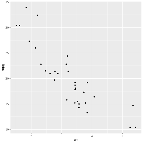
在散佈圖中,關聯性看起來似乎是線性的,而變異數看起來則為常數。 我們來嘗試使用線性迴歸建立此模型。
library(tidymodels)

# split test and training dataset
set.seed(123)
split <- initial_split(mtcars, prop = 0.7, strata = "cyl")
train <- training(split)
test <- testing(split)


# config the linear regression model
lm_spec <- linear_reg() %>%
  set_engine("lm") %>%
  set_mode("regression")

# build the model
lm_fit <- lm_spec %>%
  fit(mpg ~ wt, data = train)

tidy(lm_fit)
套用線性迴歸模型來預測測試資料集。
# using the lm model to predict on test dataset
predictions <- predict(lm_fit, test)
predictions
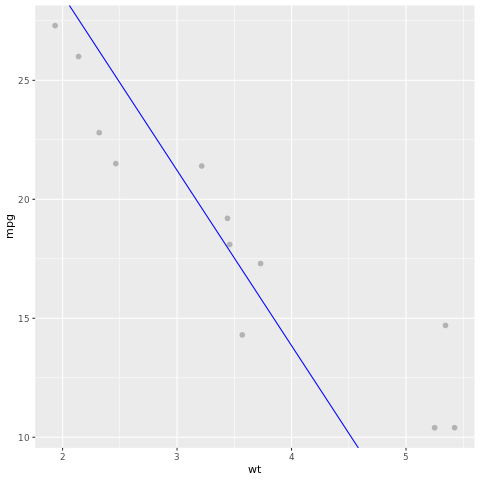
我們來看看模型結果。 我們可以將模型繪製為折線圖,並將測試的有根據事實資料繪製為相同圖表上的點。 模型看起來不錯。
# draw the model as a line chart and the test data groundtruth as points
lm_aug <- augment(lm_fit, test)
ggplot(lm_aug, aes(x = wt, y = mpg)) +
  geom_point(size=2,color="grey70") +
  geom_abline(intercept = lm_fit$fit$coefficients[1], slope = lm_fit$fit$coefficients[2], color = "blue")