Verschillende manieren om de resource-estimator uit te voeren
In dit artikel leert u hoe u kunt werken met de Azure Quantum Resource Estimator. De resource-estimator helpt u bij het schatten van de resources die nodig zijn om een kwantumprogramma uit te voeren op een kwantumcomputer. U kunt de resource-estimator gebruiken om het aantal qubits, het aantal poorten en de diepte van het circuit te schatten dat nodig is om een kwantumprogramma uit te voeren.
De Resource Estimator is beschikbaar in Visual Studio Code met de Quantum Development Kit-extensie. Zie De Quantum Development Kit installerenvoor meer informatie.
Waarschuwing
De Resource Estimator in Azure Portal is niet langer ondersteund. Je wordt aangeraden over te stappen naar de lokale Resource Estimator in Visual Studio Code, die wordt voorzien in de Quantum Development Kit.
Vereisten voor VS Code
- De nieuwste versie van Visual Studio Code of open VS Code op het web.
- De nieuwste versie van de Quantum Development Kit-extensie. Zie De QDK-extensie instellenvoor installatiedetails.
Tip
U hoeft geen Azure-account te hebben om de resource-estimator uit te voeren.
Een nieuw Q#-bestand maken
- Open Visual Studio Code en selecteer Bestand > nieuw tekstbestand om een nieuw bestand te maken.
- Sla het bestand op als
ShorRE.qs. Dit bestand bevat de Q#-code voor uw programma.
Het kwantumalgoritmen maken
Kopieer de volgende code naar het ShorRE.qs bestand:
    import Std.Arrays.*;
    import Std.Canon.*;
    import Std.Convert.*;
    import Std.Diagnostics.*;
    import Std.Math.*;
    import Std.Measurement.*;
    import Microsoft.Quantum.Unstable.Arithmetic.*;
    import Std.ResourceEstimation.*;

    operation Main() : Unit {
        let bitsize = 31;

        // When choosing parameters for `EstimateFrequency`, make sure that
        // generator and modules are not co-prime
        let _ = EstimateFrequency(11, 2^bitsize - 1, bitsize);
    }

    // In this sample we concentrate on costing the `EstimateFrequency`
    // operation, which is the core quantum operation in Shors algorithm, and
    // we omit the classical pre- and post-processing.

    /// # Summary
    /// Estimates the frequency of a generator
    /// in the residue ring Z mod `modulus`.
    ///
    /// # Input
    /// ## generator
    /// The unsigned integer multiplicative order (period)
    /// of which is being estimated. Must be co-prime to `modulus`.
    /// ## modulus
    /// The modulus which defines the residue ring Z mod `modulus`
    /// in which the multiplicative order of `generator` is being estimated.
    /// ## bitsize
    /// Number of bits needed to represent the modulus.
    ///
    /// # Output
    /// The numerator k of dyadic fraction k/2^bitsPrecision
    /// approximating s/r.
    operation EstimateFrequency(
        generator : Int,
        modulus : Int,
        bitsize : Int
    )
    : Int {
        mutable frequencyEstimate = 0;
        let bitsPrecision =  2 * bitsize + 1;

        // Allocate qubits for the superposition of eigenstates of
        // the oracle that is used in period finding.
        use eigenstateRegister = Qubit[bitsize];

        // Initialize eigenstateRegister to 1, which is a superposition of
        // the eigenstates we are estimating the phases of.
        // We first interpret the register as encoding an unsigned integer
        // in little endian encoding.
        ApplyXorInPlace(1, eigenstateRegister);
        let oracle = ApplyOrderFindingOracle(generator, modulus, _, _);

        // Use phase estimation with a semiclassical Fourier transform to
        // estimate the frequency.
        use c = Qubit();
        for idx in bitsPrecision - 1..-1..0 {
            within {
                H(c);
            } apply {
                // `BeginEstimateCaching` and `EndEstimateCaching` are the operations
                // exposed by Azure Quantum Resource Estimator. These will instruct
                // resource counting such that the if-block will be executed
                // only once, its resources will be cached, and appended in
                // every other iteration.
                if BeginEstimateCaching("ControlledOracle", SingleVariant()) {
                    Controlled oracle([c], (1 <<< idx, eigenstateRegister));
                    EndEstimateCaching();
                }
                R1Frac(frequencyEstimate, bitsPrecision - 1 - idx, c);
            }
            if MResetZ(c) == One {
                frequencyEstimate += 1 <<< (bitsPrecision - 1 - idx);
            }
        }

        // Return all the qubits used for oracles eigenstate back to 0 state
        // using Microsoft.Quantum.Intrinsic.ResetAll.
        ResetAll(eigenstateRegister);

        return frequencyEstimate;
    }

    /// # Summary
    /// Interprets `target` as encoding unsigned little-endian integer k
    /// and performs transformation |k⟩ ↦ |gᵖ⋅k mod N ⟩ where
    /// p is `power`, g is `generator` and N is `modulus`.
    ///
    /// # Input
    /// ## generator
    /// The unsigned integer multiplicative order ( period )
    /// of which is being estimated. Must be co-prime to `modulus`.
    /// ## modulus
    /// The modulus which defines the residue ring Z mod `modulus`
    /// in which the multiplicative order of `generator` is being estimated.
    /// ## power
    /// Power of `generator` by which `target` is multiplied.
    /// ## target
    /// Register interpreted as little endian encoded which is multiplied by
    /// given power of the generator. The multiplication is performed modulo
    /// `modulus`.
    internal operation ApplyOrderFindingOracle(
        generator : Int, modulus : Int, power : Int, target : Qubit[]
    )
    : Unit
    is Adj + Ctl {
        // The oracle we use for order finding implements |x⟩ ↦ |x⋅a mod N⟩. We
        // also use `ExpModI` to compute a by which x must be multiplied. Also
        // note that we interpret target as unsigned integer in little-endian
        // encoding.
        ModularMultiplyByConstant(modulus,
                                    ExpModI(generator, power, modulus),
                                    target);
    }

    /// # Summary
    /// Performs modular in-place multiplication by a classical constant.
    ///
    /// # Description
    /// Given the classical constants `c` and `modulus`, and an input
    /// quantum register  |𝑦⟩, this operation
    /// computes `(c*x) % modulus` into |𝑦⟩.
    ///
    /// # Input
    /// ## modulus
    /// Modulus to use for modular multiplication
    /// ## c
    /// Constant by which to multiply |𝑦⟩
    /// ## y
    /// Quantum register of target
    internal operation ModularMultiplyByConstant(modulus : Int, c : Int, y : Qubit[])
    : Unit is Adj + Ctl {
        use qs = Qubit[Length(y)];
        for (idx, yq) in Enumerated(y) {
            let shiftedC = (c <<< idx) % modulus;
            Controlled ModularAddConstant([yq], (modulus, shiftedC, qs));
        }
        ApplyToEachCA(SWAP, Zipped(y, qs));
        let invC = InverseModI(c, modulus);
        for (idx, yq) in Enumerated(y) {
            let shiftedC = (invC <<< idx) % modulus;
            Controlled ModularAddConstant([yq], (modulus, modulus - shiftedC, qs));
        }
    }

    /// # Summary
    /// Performs modular in-place addition of a classical constant into a
    /// quantum register.
    ///
    /// # Description
    /// Given the classical constants `c` and `modulus`, and an input
    /// quantum register  |𝑦⟩, this operation
    /// computes `(x+c) % modulus` into |𝑦⟩.
    ///
    /// # Input
    /// ## modulus
    /// Modulus to use for modular addition
    /// ## c
    /// Constant to add to |𝑦⟩
    /// ## y
    /// Quantum register of target
    internal operation ModularAddConstant(modulus : Int, c : Int, y : Qubit[])
    : Unit is Adj + Ctl {
        body (...) {
            Controlled ModularAddConstant([], (modulus, c, y));
        }
        controlled (ctrls, ...) {
            // We apply a custom strategy to control this operation instead of
            // letting the compiler create the controlled variant for us in which
            // the `Controlled` functor would be distributed over each operation
            // in the body.
            //
            // Here we can use some scratch memory to save ensure that at most one
            // control qubit is used for costly operations such as `AddConstant`
            // and `CompareGreaterThenOrEqualConstant`.
            if Length(ctrls) >= 2 {
                use control = Qubit();
                within {
                    Controlled X(ctrls, control);
                } apply {
                    Controlled ModularAddConstant([control], (modulus, c, y));
                }
            } else {
                use carry = Qubit();
                Controlled AddConstant(ctrls, (c, y + [carry]));
                Controlled Adjoint AddConstant(ctrls, (modulus, y + [carry]));
                Controlled AddConstant([carry], (modulus, y));
                Controlled CompareGreaterThanOrEqualConstant(ctrls, (c, y, carry));
            }
        }
    }

    /// # Summary
    /// Performs in-place addition of a constant into a quantum register.
    ///
    /// # Description
    /// Given a non-empty quantum register |𝑦⟩ of length 𝑛+1 and a positive
    /// constant 𝑐 < 2ⁿ, computes |𝑦 + c⟩ into |𝑦⟩.
    ///
    /// # Input
    /// ## c
    /// Constant number to add to |𝑦⟩.
    /// ## y
    /// Quantum register of second summand and target; must not be empty.
    internal operation AddConstant(c : Int, y : Qubit[]) : Unit is Adj + Ctl {
        // We are using this version instead of the library version that is based
        // on Fourier angles to show an advantage of sparse simulation in this sample.

        let n = Length(y);
        Fact(n > 0, "Bit width must be at least 1");

        Fact(c >= 0, "constant must not be negative");
        Fact(c < 2 ^ n, $"constant must be smaller than {2L ^ n}");

        if c != 0 {
            // If c has j trailing zeroes than the j least significant bits
            // of y won't be affected by the addition and can therefore be
            // ignored by applying the addition only to the other qubits and
            // shifting c accordingly.
            let j = NTrailingZeroes(c);
            use x = Qubit[n - j];
            within {
                ApplyXorInPlace(c >>> j, x);
            } apply {
                IncByLE(x, y[j...]);
            }
        }
    }

    /// # Summary
    /// Performs greater-than-or-equals comparison to a constant.
    ///
    /// # Description
    /// Toggles output qubit `target` if and only if input register `x`
    /// is greater than or equal to `c`.
    ///
    /// # Input
    /// ## c
    /// Constant value for comparison.
    /// ## x
    /// Quantum register to compare against.
    /// ## target
    /// Target qubit for comparison result.
    ///
    /// # Reference
    /// This construction is described in [Lemma 3, arXiv:2201.10200]
    internal operation CompareGreaterThanOrEqualConstant(c : Int, x : Qubit[], target : Qubit)
    : Unit is Adj+Ctl {
        let bitWidth = Length(x);

        if c == 0 {
            X(target);
        } elif c >= 2 ^ bitWidth {
            // do nothing
        } elif c == 2 ^ (bitWidth - 1) {
            ApplyLowTCNOT(Tail(x), target);
        } else {
            // normalize constant
            let l = NTrailingZeroes(c);

            let cNormalized = c >>> l;
            let xNormalized = x[l...];
            let bitWidthNormalized = Length(xNormalized);
            let gates = Rest(IntAsBoolArray(cNormalized, bitWidthNormalized));

            use qs = Qubit[bitWidthNormalized - 1];
            let cs1 = [Head(xNormalized)] + Most(qs);
            let cs2 = Rest(xNormalized);

            within {
                for i in IndexRange(gates) {
                    (gates[i] ? ApplyAnd | ApplyOr)(cs1[i], cs2[i], qs[i]);
                }
            } apply {
                ApplyLowTCNOT(Tail(qs), target);
            }
        }
    }

    /// # Summary
    /// Internal operation used in the implementation of GreaterThanOrEqualConstant.
    internal operation ApplyOr(control1 : Qubit, control2 : Qubit, target : Qubit) : Unit is Adj {
        within {
            ApplyToEachA(X, [control1, control2]);
        } apply {
            ApplyAnd(control1, control2, target);
            X(target);
        }
    }

    internal operation ApplyAnd(control1 : Qubit, control2 : Qubit, target : Qubit)
    : Unit is Adj {
        body (...) {
            CCNOT(control1, control2, target);
        }
        adjoint (...) {
            H(target);
            if (M(target) == One) {
                X(target);
                CZ(control1, control2);
            }
        }
    }


    /// # Summary
    /// Returns the number of trailing zeroes of a number
    ///
    /// ## Example
    /// ```qsharp
    /// let zeroes = NTrailingZeroes(21); // = NTrailingZeroes(0b1101) = 0
    /// let zeroes = NTrailingZeroes(20); // = NTrailingZeroes(0b1100) = 2
    /// ```
    internal function NTrailingZeroes(number : Int) : Int {
        mutable nZeroes = 0;
        mutable copy = number;
        while (copy % 2 == 0) {
            nZeroes += 1;
            copy /= 2;
        }
        return nZeroes;
    }

    /// # Summary
    /// An implementation for `CNOT` that when controlled using a single control uses
    /// a helper qubit and uses `ApplyAnd` to reduce the T-count to 4 instead of 7.
    internal operation ApplyLowTCNOT(a : Qubit, b : Qubit) : Unit is Adj+Ctl {
        body (...) {
            CNOT(a, b);
        }

        adjoint self;

        controlled (ctls, ...) {
            // In this application this operation is used in a way that
            // it is controlled by at most one qubit.
            Fact(Length(ctls) <= 1, "At most one control line allowed");

            if IsEmpty(ctls) {
                CNOT(a, b);
            } else {
                use q = Qubit();
                within {
                    ApplyAnd(Head(ctls), a, q);
                } apply {
                    CNOT(q, b);
                }
            }
        }

        controlled adjoint self;
    }
De resource-estimator uitvoeren
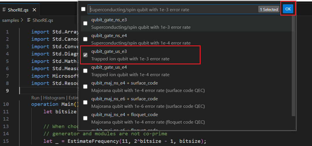
De Resource Estimator biedt zes vooraf gedefinieerde qubitparameters, waarvan vier op poorten gebaseerde instructiesets en twee met een Majorana-instructieset. Het biedt ook twee kwantumfoutcorrectiecodes, surface_code en floquet_code.
In dit voorbeeld voert u de resource-estimator uit met behulp van de qubit_gate_us_e3 qubitparameter en de code voor kwantumfoutcorrectie surface_code .
Selecteer Weergave -> opdrachtpalet en typ 'resource' die de optie Q#: Resourceschattingen berekenen moet worden weergegeven. U kunt ook klikken op Schatting in de lijst met opdrachten die direct vóór de
Mainbewerking worden weergegeven. Selecteer deze optie om het venster Resource-estimator te openen.
U kunt een of meer qubitparameter en foutcodetypen selecteren om de resources voor te schatten. Selecteer voor dit voorbeeld qubit_gate_us_e3 en klik op OK.
Geef het foutbudget op of accepteer de standaardwaarde 0,001. Laat voor dit voorbeeld de standaardwaarde staan en druk op Enter.
Druk op Enter om de standaardresultaatnaam te accepteren op basis van de bestandsnaam, in dit geval ShorRE.
De resultaten bekijken
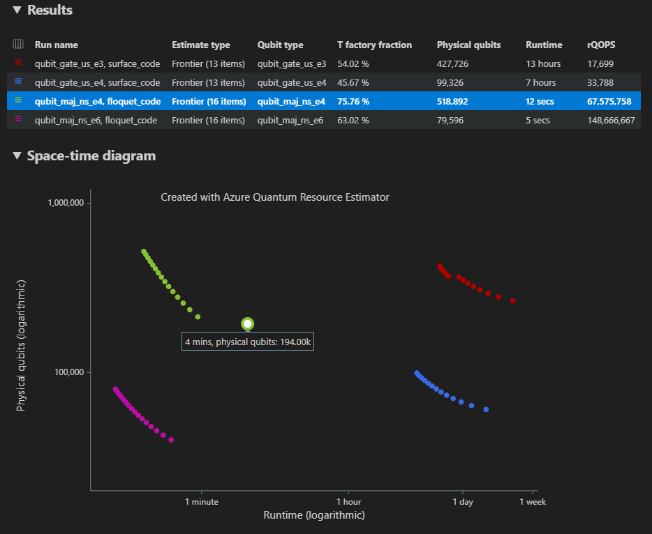
De resource-estimator biedt meerdere schattingen voor hetzelfde algoritme, elk met compromissen tussen het aantal qubits en de runtime. Inzicht in de balans tussen runtime en systeemschaal is een van de belangrijkste aspecten van de schatting van resources.
Het resultaat van de schatting van de resource wordt weergegeven in het Q#-schattingsvenster .
Op het tabblad Resultaten wordt een samenvatting van de schatting van de resource weergegeven. Klik op het pictogram naast de eerste rij om de kolommen te selecteren die u wilt weergeven. U kunt kiezen uit de uitvoeringsnaam, het schattingstype, het qubittype, het qec-schema, het foutbudget, logische qubits, logische diepte, codeafstand, T-statussen, T-factory's, T factory-breuk, runtime, rQOPS en fysieke qubits.
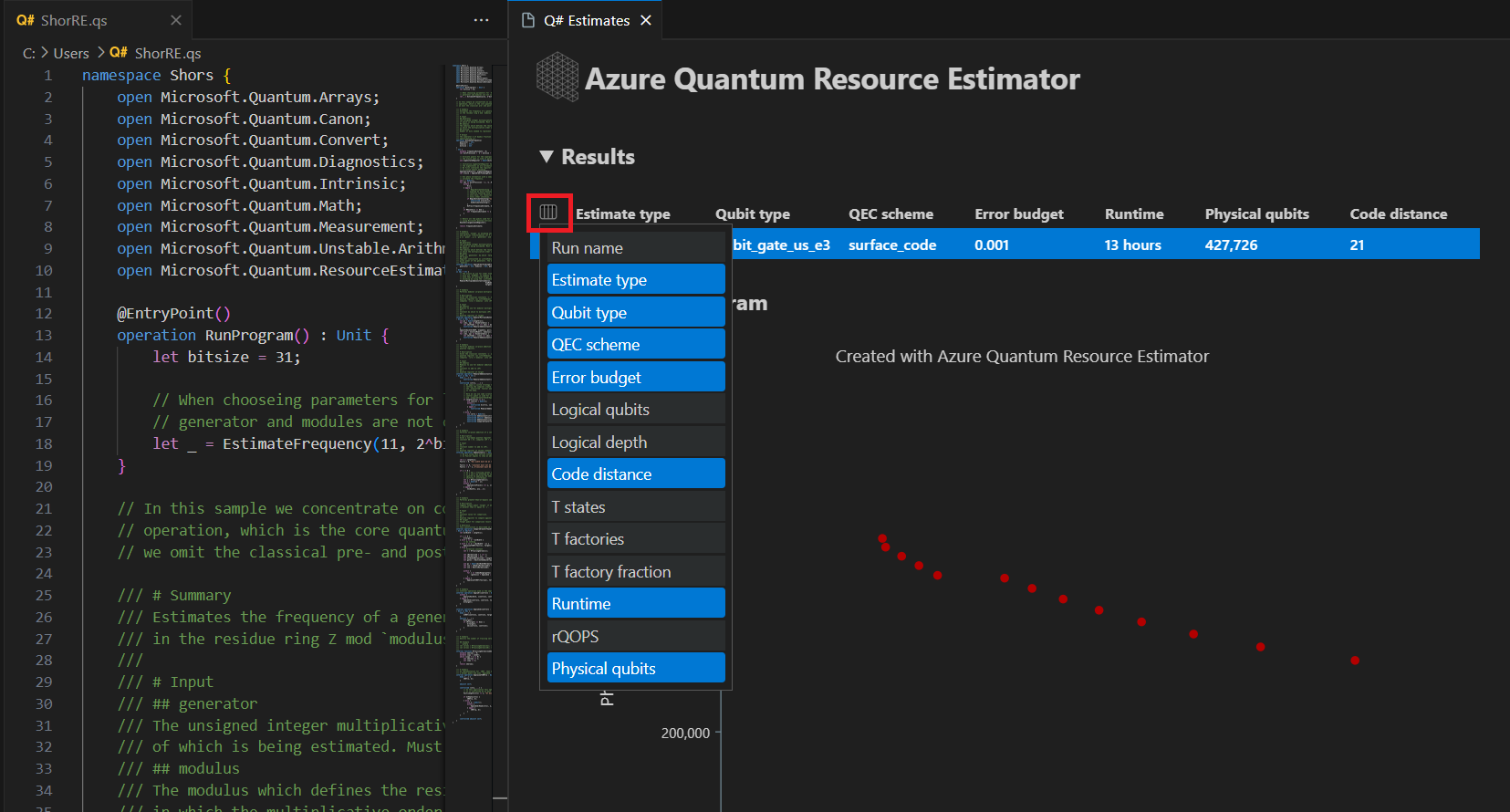
In de kolom Schattingstype van de resultatentabel ziet u het aantal optimale combinaties van {aantal qubits, runtime} voor uw algoritme. Deze combinaties zijn te zien in het ruimte-tijddiagram.
In het diagram ruimtetijd ziet u de afwegingen tussen het aantal fysieke qubits en de runtime van het algoritme. In dit geval vindt de resource-estimator 13 verschillende optimale combinaties van vele duizenden mogelijke combinaties. U kunt de muisaanwijzer op elk {aantal qubits, runtime}-punt bewegen om de details van de schatting van de resource op dat moment te bekijken.
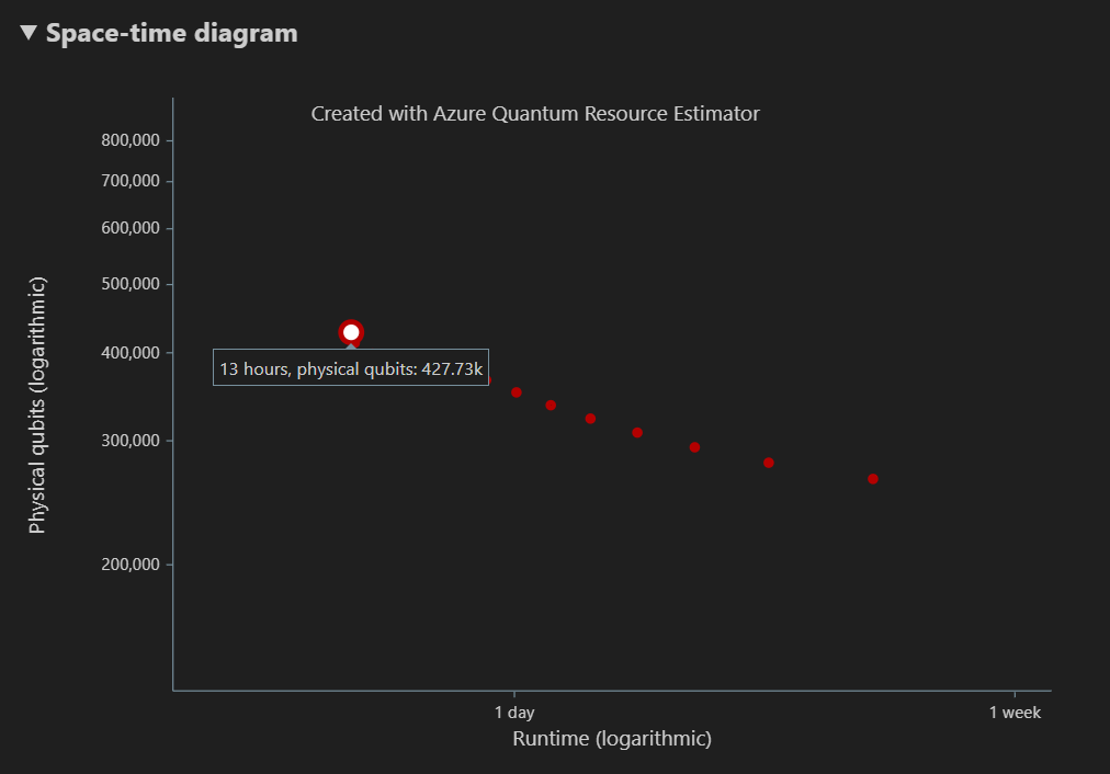
Zie het diagram ruimtetijd voor meer informatie.
Notitie
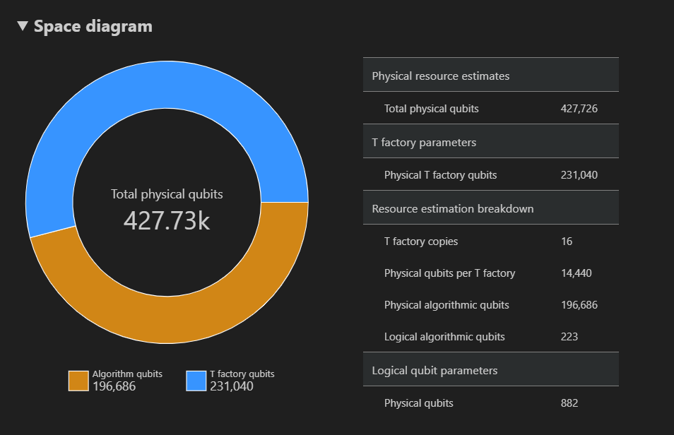
U moet op één punt van het tijddiagram klikken, dat een {aantal qubits, runtime}-paar is, om het ruimtediagram en de details van de resourceraming te zien die overeenkomt met dat punt.
In het ruimtediagram ziet u de verdeling van fysieke qubits die worden gebruikt voor het algoritme en de T-factory's, die overeenkomen met een {aantal qubits, runtime}-paar. Als u bijvoorbeeld het meest linkse punt in het tijddiagram selecteert, zijn het aantal fysieke qubits dat nodig is om het algoritme uit te voeren 427726, 196686 algoritme-qubits zijn en waarvan 231040 T factory-qubits zijn.
Ten slotte bevat het tabblad Resourceschattingen de volledige lijst met uitvoergegevens voor de Resource-estimator die overeenkomt met een {aantal qubits, runtime} -paar. U kunt kostendetails inspecteren door de groepen samen te vouwen, die meer informatie hebben. Selecteer bijvoorbeeld het meest linkse punt in het ruimtetijddiagram en vouw de groep logische qubitparameters samen.
Parameter logische qubit Weergegeven als QEC-schema surface_code Codeafstand 21 Fysieke qubits 882 Tijd van logische cyclus 13 millisecs Foutpercentage logische qubit 3.00E-13 Kruising vooraf 0.03 Drempelwaarde voor foutcorrectie 0,01 Formule voor tijd van logische cyclus (4 * twoQubitGateTime+ 2 *oneQubitMeasurementTime) * *codeDistanceFormule voor fysieke qubits 2 * codeDistance*codeDistanceTip
Klik op Gedetailleerde rijen weergeven om de beschrijving van elke uitvoer van de rapportgegevens weer te geven.
Zie de volledige rapportgegevens van de resource-estimator voor meer informatie.
target De parameters wijzigen
U kunt de kosten voor hetzelfde Q#-programma schatten met behulp van een ander qubittype, foutcorrectiecode en foutbudget. Open het venster Resource-estimator door Weergave - Opdrachtpalet>en typ .Q#: Calculate Resource Estimates
Selecteer een andere configuratie, bijvoorbeeld de op Majorana gebaseerde qubitparameter. qubit_maj_ns_e6 Accepteer de standaardwaarde van het foutbudget of voer een nieuwe in en druk op Enter. De resource-estimator voert de schatting opnieuw uit met de nieuwe target parameters.
Zie Target de parameters voor de resource-estimator voor meer informatie.
Meerdere configuraties van parameters uitvoeren
De Azure Quantum Resource Estimator kan meerdere configuraties van parameters uitvoeren en de resultaten van target de resourceraming vergelijken.
Selecteer Weergave -> Opdrachtpalet of druk op Ctrl+Shift+P en typ
Q#: Calculate Resource Estimates.Selecteer qubit_gate_us_e3, qubit_gate_us_e4, qubit_maj_ns_e4 + floquet_code en qubit_maj_ns_e6 + floquet_code en klik op OK.
Accepteer de standaardfoutbudgetwaarde 0,001 en druk op Enter.
Druk op Enter om het invoerbestand te accepteren, in dit geval ShorRE.qs.
In het geval van meerdere configuraties van parameters worden de resultaten weergegeven in verschillende rijen op het tabblad Resultaten .
In het diagram Ruimtetijd ziet u de resultaten voor alle configuraties van parameters. In de eerste kolom van de resultatentabel wordt de legenda weergegeven voor elke configuratie van parameters. U kunt de muisaanwijzer op elk punt bewegen om de details van de schatting van de resource op dat moment weer te geven.
Klik op een {aantal qubits, runtime} punt van het ruimte-tijddiagram om het bijbehorende ruimtediagram en rapportgegevens weer te geven.
Vereisten voor Jupyter Notebook in VS Code
Een Python-omgeving waarop Python en Pip zijn geïnstalleerd.
De nieuwste versie van Visual Studio Code of open VS Code op het web.
VS Code met de Quantum Development Kit, Pythonen Jupyter-extensies geïnstalleerd.
De nieuwste Azure Quantum
qsharpenqsharp_widgetspakketten.python -m pip install --upgrade qsharp qsharp_widgetsof
!pip install --upgrade qsharp qsharp_widgets
Tip
U hoeft geen Azure-account te hebben om de resource-estimator uit te voeren.
Het kwantumalgoritmen maken
Selecteer in VS Code het > Weergeven en selecteer Maken: Nieuw Jupyter Notebook.
In de rechterbovenhoek detecteert en geeft VS Code de versie van Python en de virtuele Python-omgeving weer die is geselecteerd voor het notebook. Als u meerdere Python-omgevingen hebt, moet u mogelijk een kernel selecteren met behulp van de kernelkiezer in de rechterbovenhoek. Als er geen omgeving is gedetecteerd, raadpleegt u Jupyter Notebooks in VS Code voor informatie over de installatie.
Importeer het
qsharppakket in de eerste cel van het notebook.import qsharpVoeg een nieuwe cel toe en kopieer de volgende code.
%%qsharp
import Std.Arrays.*;
import Std.Canon.*;
import Std.Convert.*;
import Std.Diagnostics.*;
import Std.Math.*;
import Std.Measurement.*;
import Microsoft.Quantum.Unstable.Arithmetic.*;
import Std.ResourceEstimation.*;

operation RunProgram() : Unit {
    let bitsize = 31;

    // When choosing parameters for `EstimateFrequency`, make sure that
    // generator and modules are not co-prime
    let _ = EstimateFrequency(11, 2^bitsize - 1, bitsize);
}


// In this sample we concentrate on costing the `EstimateFrequency`
// operation, which is the core quantum operation in Shors algorithm, and
// we omit the classical pre- and post-processing.

/// # Summary
/// Estimates the frequency of a generator
/// in the residue ring Z mod `modulus`.
///
/// # Input
/// ## generator
/// The unsigned integer multiplicative order (period)
/// of which is being estimated. Must be co-prime to `modulus`.
/// ## modulus
/// The modulus which defines the residue ring Z mod `modulus`
/// in which the multiplicative order of `generator` is being estimated.
/// ## bitsize
/// Number of bits needed to represent the modulus.
///
/// # Output
/// The numerator k of dyadic fraction k/2^bitsPrecision
/// approximating s/r.
operation EstimateFrequency(
    generator : Int,
    modulus : Int,
    bitsize : Int
)
: Int {
    mutable frequencyEstimate = 0;
    let bitsPrecision =  2 * bitsize + 1;

    // Allocate qubits for the superposition of eigenstates of
    // the oracle that is used in period finding.
    use eigenstateRegister = Qubit[bitsize];

    // Initialize eigenstateRegister to 1, which is a superposition of
    // the eigenstates we are estimating the phases of.
    // We first interpret the register as encoding an unsigned integer
    // in little endian encoding.
    ApplyXorInPlace(1, eigenstateRegister);
    let oracle = ApplyOrderFindingOracle(generator, modulus, _, _);

    // Use phase estimation with a semiclassical Fourier transform to
    // estimate the frequency.
    use c = Qubit();
    for idx in bitsPrecision - 1..-1..0 {
        within {
            H(c);
        } apply {
            // `BeginEstimateCaching` and `EndEstimateCaching` are the operations
            // exposed by Azure Quantum Resource Estimator. These will instruct
            // resource counting such that the if-block will be executed
            // only once, its resources will be cached, and appended in
            // every other iteration.
            if BeginEstimateCaching("ControlledOracle", SingleVariant()) {
                Controlled oracle([c], (1 <<< idx, eigenstateRegister));
                EndEstimateCaching();
            }
            R1Frac(frequencyEstimate, bitsPrecision - 1 - idx, c);
        }
        if MResetZ(c) == One {
            frequencyEstimate += 1 <<< (bitsPrecision - 1 - idx);
        }
    }

    // Return all the qubits used for oracle eigenstate back to 0 state
    // using Microsoft.Quantum.Intrinsic.ResetAll.
    ResetAll(eigenstateRegister);

    return frequencyEstimate;
}

/// # Summary
/// Interprets `target` as encoding unsigned little-endian integer k
/// and performs transformation |k⟩ ↦ |gᵖ⋅k mod N ⟩ where
/// p is `power`, g is `generator` and N is `modulus`.
///
/// # Input
/// ## generator
/// The unsigned integer multiplicative order ( period )
/// of which is being estimated. Must be co-prime to `modulus`.
/// ## modulus
/// The modulus which defines the residue ring Z mod `modulus`
/// in which the multiplicative order of `generator` is being estimated.
/// ## power
/// Power of `generator` by which `target` is multiplied.
/// ## target
/// Register interpreted as little endian encoded which is multiplied by
/// given power of the generator. The multiplication is performed modulo
/// `modulus`.
internal operation ApplyOrderFindingOracle(
    generator : Int, modulus : Int, power : Int, target : Qubit[]
)
: Unit
is Adj + Ctl {
    // The oracle we use for order finding implements |x⟩ ↦ |x⋅a mod N⟩. We
    // also use `ExpModI` to compute a by which x must be multiplied. Also
    // note that we interpret target as unsigned integer in little-endian
    // encoding.
    ModularMultiplyByConstant(modulus,
                                ExpModI(generator, power, modulus),
                                target);
}

/// # Summary
/// Performs modular in-place multiplication by a classical constant.
///
/// # Description
/// Given the classical constants `c` and `modulus`, and an input
/// quantum register |𝑦⟩, this operation
/// computes `(c*x) % modulus` into |𝑦⟩.
///
/// # Input
/// ## modulus
/// Modulus to use for modular multiplication
/// ## c
/// Constant by which to multiply |𝑦⟩
/// ## y
/// Quantum register of target
internal operation ModularMultiplyByConstant(modulus : Int, c : Int, y : Qubit[])
: Unit is Adj + Ctl {
    use qs = Qubit[Length(y)];
    for (idx, yq) in Enumerated(y) {
        let shiftedC = (c <<< idx) % modulus;
        Controlled ModularAddConstant([yq], (modulus, shiftedC, qs));
    }
    ApplyToEachCA(SWAP, Zipped(y, qs));
    let invC = InverseModI(c, modulus);
    for (idx, yq) in Enumerated(y) {
        let shiftedC = (invC <<< idx) % modulus;
        Controlled ModularAddConstant([yq], (modulus, modulus - shiftedC, qs));
    }
}

/// # Summary
/// Performs modular in-place addition of a classical constant into a
/// quantum register.
///
/// # Description
/// Given the classical constants `c` and `modulus`, and an input
/// quantum register  |𝑦⟩, this operation
/// computes `(x+c) % modulus` into |𝑦⟩.
///
/// # Input
/// ## modulus
/// Modulus to use for modular addition
/// ## c
/// Constant to add to |𝑦⟩
/// ## y
/// Quantum register of target
internal operation ModularAddConstant(modulus : Int, c : Int, y : Qubit[])
: Unit is Adj + Ctl {
    body (...) {
        Controlled ModularAddConstant([], (modulus, c, y));
    }
    controlled (ctrls, ...) {
        // We apply a custom strategy to control this operation instead of
        // letting the compiler create the controlled variant for us in which
        // the `Controlled` functor would be distributed over each operation
        // in the body.
        //
        // Here we can use some scratch memory to save ensure that at most one
        // control qubit is used for costly operations such as `AddConstant`
        // and `CompareGreaterThenOrEqualConstant`.
        if Length(ctrls) >= 2 {
            use control = Qubit();
            within {
                Controlled X(ctrls, control);
            } apply {
                Controlled ModularAddConstant([control], (modulus, c, y));
            }
        } else {
            use carry = Qubit();
            Controlled AddConstant(ctrls, (c, y + [carry]));
            Controlled Adjoint AddConstant(ctrls, (modulus, y + [carry]));
            Controlled AddConstant([carry], (modulus, y));
            Controlled CompareGreaterThanOrEqualConstant(ctrls, (c, y, carry));
        }
    }
}

/// # Summary
/// Performs in-place addition of a constant into a quantum register.
///
/// # Description
/// Given a non-empty quantum register |𝑦⟩ of length 𝑛+1 and a positive
/// constant 𝑐 < 2ⁿ, computes |𝑦 + c⟩ into |𝑦⟩.
///
/// # Input
/// ## c
/// Constant number to add to |𝑦⟩.
/// ## y
/// Quantum register of second summand and target; must not be empty.
internal operation AddConstant(c : Int, y : Qubit[]) : Unit is Adj + Ctl {
    // We are using this version instead of the library version that is based
    // on Fourier angles to show an advantage of sparse simulation in this sample.

    let n = Length(y);
    Fact(n > 0, "Bit width must be at least 1");

    Fact(c >= 0, "constant must not be negative");
    Fact(c < 2 ^ n, $"constant must be smaller than {2L ^ n}");

    if c != 0 {
        // If c has j trailing zeroes than the j least significant bits
        // of y will not be affected by the addition and can therefore be
        // ignored by applying the addition only to the other qubits and
        // shifting c accordingly.
        let j = NTrailingZeroes(c);
        use x = Qubit[n - j];
        within {
            ApplyXorInPlace(c >>> j, x);
        } apply {
            IncByLE(x, y[j...]);
        }
    }
}

/// # Summary
/// Performs greater-than-or-equals comparison to a constant.
///
/// # Description
/// Toggles output qubit `target` if and only if input register `x`
/// is greater than or equal to `c`.
///
/// # Input
/// ## c
/// Constant value for comparison.
/// ## x
/// Quantum register to compare against.
/// ## target
/// Target qubit for comparison result.
///
/// # Reference
/// This construction is described in [Lemma 3, arXiv:2201.10200]
internal operation CompareGreaterThanOrEqualConstant(c : Int, x : Qubit[], target : Qubit)
: Unit is Adj+Ctl {
    let bitWidth = Length(x);

    if c == 0 {
        X(target);
    } elif c >= 2 ^ bitWidth {
        // do nothing
    } elif c == 2 ^ (bitWidth - 1) {
        ApplyLowTCNOT(Tail(x), target);
    } else {
        // normalize constant
        let l = NTrailingZeroes(c);

        let cNormalized = c >>> l;
        let xNormalized = x[l...];
        let bitWidthNormalized = Length(xNormalized);
        let gates = Rest(IntAsBoolArray(cNormalized, bitWidthNormalized));

        use qs = Qubit[bitWidthNormalized - 1];
        let cs1 = [Head(xNormalized)] + Most(qs);
        let cs2 = Rest(xNormalized);

        within {
            for i in IndexRange(gates) {
                (gates[i] ? ApplyAnd | ApplyOr)(cs1[i], cs2[i], qs[i]);
            }
        } apply {
            ApplyLowTCNOT(Tail(qs), target);
        }
    }
}

/// # Summary
/// Internal operation used in the implementation of GreaterThanOrEqualConstant.
internal operation ApplyOr(control1 : Qubit, control2 : Qubit, target : Qubit) : Unit is Adj {
    within {
        ApplyToEachA(X, [control1, control2]);
    } apply {
        ApplyAnd(control1, control2, target);
        X(target);
    }
}

internal operation ApplyAnd(control1 : Qubit, control2 : Qubit, target : Qubit)
: Unit is Adj {
    body (...) {
        CCNOT(control1, control2, target);
    }
    adjoint (...) {
        H(target);
        if (M(target) == One) {
            X(target);
            CZ(control1, control2);
        }
    }
}


/// # Summary
/// Returns the number of trailing zeroes of a number
///
/// ## Example
/// ```qsharp
/// let zeroes = NTrailingZeroes(21); // = NTrailingZeroes(0b1101) = 0
/// let zeroes = NTrailingZeroes(20); // = NTrailingZeroes(0b1100) = 2
/// ```
internal function NTrailingZeroes(number : Int) : Int {
    mutable nZeroes = 0;
    mutable copy = number;
    while (copy % 2 == 0) {
        nZeroes += 1;
        copy /= 2;
    }
    return nZeroes;
}

/// # Summary
/// An implementation for `CNOT` that when controlled using a single control uses
/// a helper qubit and uses `ApplyAnd` to reduce the T-count to 4 instead of 7.
internal operation ApplyLowTCNOT(a : Qubit, b : Qubit) : Unit is Adj+Ctl {
    body (...) {
        CNOT(a, b);
    }

    adjoint self;

    controlled (ctls, ...) {
        // In this application this operation is used in a way that
        // it is controlled by at most one qubit.
        Fact(Length(ctls) <= 1, "At most one control line allowed");

        if IsEmpty(ctls) {
            CNOT(a, b);
        } else {
            use q = Qubit();
            within {
                ApplyAnd(Head(ctls), a, q);
            } apply {
                CNOT(q, b);
            }
        }
    }

    controlled adjoint self;
}
Het kwantumalgoritmen schatten
Nu maakt u een schatting van de fysieke resources voor de RunProgram bewerking met behulp van de standaardveronderstellingen. Voeg een nieuwe cel toe en kopieer de volgende code.
result = qsharp.estimate("RunProgram()")
result
De qsharp.estimate functie maakt een resultaatobject, dat kan worden gebruikt om een tabel weer te geven met het totale aantal fysieke resources. U kunt kostendetails inspecteren door de groepen uit te vouwen, die meer informatie hebben. Zie de volledige rapportgegevens van de resource-estimator voor meer informatie.
Vouw bijvoorbeeld de logische qubitparameters uit groep om te zien dat de codeafstand 21 is en het aantal fysieke qubits 882 is.
| Parameter logische qubit | Weergegeven als |
|---|---|
| QEC-schema | surface_code |
| Codeafstand | 21 |
| Fysieke qubits | 882 |
| Tijd van logische cyclus | 8 millisecs |
| Foutpercentage logische qubit | 3.00E-13 |
| Kruising vooraf | 0.03 |
| Drempelwaarde voor foutcorrectie | 0,01 |
| Formule voor tijd van logische cyclus | (4 * twoQubitGateTime + 2 * oneQubitMeasurementTime) * * codeDistance |
| Formule voor fysieke qubits | 2 * codeDistance * codeDistance |
Tip
Voor een compactere versie van de uitvoertabel kunt u deze gebruiken result.summary.
Ruimtediagram
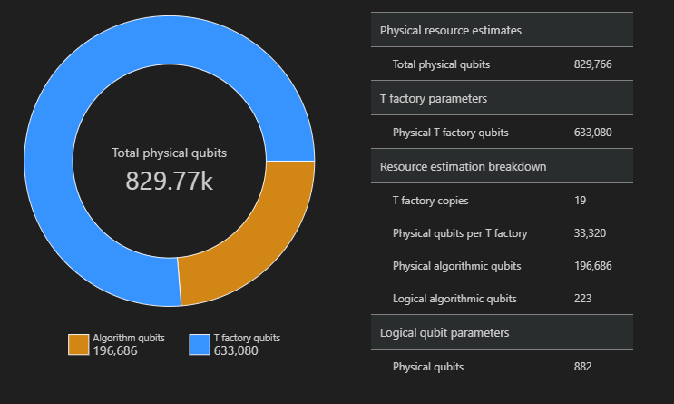
De verdeling van fysieke qubits die worden gebruikt voor het algoritme en de T-factory's is een factor die van invloed kan zijn op het ontwerp van uw algoritme. U kunt het qsharp-widgets pakket gebruiken om deze distributie te visualiseren om meer inzicht te krijgen in de geschatte ruimtevereisten voor het algoritme.
from qsharp-widgets import SpaceChart, EstimateDetails
SpaceChart(result)
In dit voorbeeld zijn het aantal fysieke qubits dat nodig is om het algoritme uit te voeren, 829766, waarvan 196686 algoritme-qubits zijn en waarvan 633080 T factory-qubits zijn.
De standaardwaarden wijzigen en het algoritme schatten
Wanneer u een aanvraag voor een resourceraming voor uw programma indient, kunt u enkele optionele parameters opgeven. Gebruik het jobParams veld om toegang te krijgen tot alle target parameters die kunnen worden doorgegeven aan de taakuitvoering en om te zien welke standaardwaarden zijn aangenomen:
result['jobParams']
{'errorBudget': 0.001,
 'qecScheme': {'crossingPrefactor': 0.03,
  'errorCorrectionThreshold': 0.01,
  'logicalCycleTime': '(4 * twoQubitGateTime + 2 * oneQubitMeasurementTime) * codeDistance',
  'name': 'surface_code',
  'physicalQubitsPerLogicalQubit': '2 * codeDistance * codeDistance'},
 'qubitParams': {'instructionSet': 'GateBased',
  'name': 'qubit_gate_ns_e3',
  'oneQubitGateErrorRate': 0.001,
  'oneQubitGateTime': '50 ns',
  'oneQubitMeasurementErrorRate': 0.001,
  'oneQubitMeasurementTime': '100 ns',
  'tGateErrorRate': 0.001,
  'tGateTime': '50 ns',
  'twoQubitGateErrorRate': 0.001,
  'twoQubitGateTime': '50 ns'}}
U kunt zien dat de Resource Estimator het qubit_gate_ns_e3 qubitmodel, de surface_code foutcode en het foutenbudget 0,001 als standaardwaarden voor de schatting gebruikt.
Dit zijn de target parameters die kunnen worden aangepast:
-
errorBudget- het totale toegestane foutbudget voor het algoritme -
qecScheme- het QEC-schema (kwantumfoutcorrectie) -
qubitParams- de parameters van de fysieke qubit -
constraints- de beperkingen op onderdeelniveau -
distillationUnitSpecifications- de specificaties voor T factory's destillatiealgoritmen -
estimateType- enkele of grens
Zie Target de parameters voor de resource-estimator voor meer informatie.
Qubitmodel wijzigen
U kunt de kosten voor hetzelfde algoritme schatten met behulp van de op Majorana gebaseerde qubitparameter, qubitParams'qubit_maj_ns_e6'.
result_maj = qsharp.estimate("RunProgram()", params={
                "qubitParams": {
                    "name": "qubit_maj_ns_e6"
                }})
EstimateDetails(result_maj)
Kwantumfoutcorrectieschema wijzigen
U kunt de resourceramingstaak opnieuw uitvoeren voor hetzelfde voorbeeld op de qubitparameters op basis van Majorana met een floqued QEC-schema. qecScheme
result_maj = qsharp.estimate("RunProgram()", params={
                "qubitParams": {
                    "name": "qubit_maj_ns_e6"
                },
                "qecScheme": {
                    "name": "floquet_code"
                }})
EstimateDetails(result_maj)
Foutbudget wijzigen
Voer vervolgens hetzelfde kwantumcircuit opnieuw uit met een errorBudget van 10%.
result_maj = qsharp.estimate("RunProgram()", params={
                "qubitParams": {
                    "name": "qubit_maj_ns_e6"
                },
                "qecScheme": {
                    "name": "floquet_code"
                },
                "errorBudget": 0.1})
EstimateDetails(result_maj)
Batchverwerking met de resource-estimator
Met de Azure Quantum Resource Estimator kunt u meerdere configuratie van target parameters uitvoeren en de resultaten vergelijken. Dit is handig als u de kosten van verschillende qubitmodellen, QEC-schema's of foutbudgetten wilt vergelijken.
U kunt een batchschatting uitvoeren door een lijst met target parameters door te geven aan de
paramsparameter van deqsharp.estimatefunctie. Voer bijvoorbeeld hetzelfde algoritme uit met de standaardparameters en de qubitparameters op basis van Majorana met een QEC-schema van floquet.result_batch = qsharp.estimate("RunProgram()", params= [{}, # Default parameters { "qubitParams": { "name": "qubit_maj_ns_e6" }, "qecScheme": { "name": "floquet_code" } }]) result_batch.summary_data_frame(labels=["Gate-based ns, 10⁻³", "Majorana ns, 10⁻⁶"])Modelleren Logische qubits Logische diepte T-statussen Codeafstand T-fabrieken T-fabrieksfractie Fysieke qubits rQOPS Fysieke runtime Poort-gebaseerde ns, 10⁻³ 223 3,64M 4,70M 21 19 76.30 % 829,77k 26,55M 31 sec. Majorana ns, 10⁻⁶ 223 3,64M 4,70M 5 19 63.02 % 79,60k 148,67M 5 sec. U kunt ook een lijst met schattingsparameters maken met behulp van de
EstimatorParamsklasse.from qsharp.estimator import EstimatorParams, QubitParams, QECScheme, LogicalCounts labels = ["Gate-based µs, 10⁻³", "Gate-based µs, 10⁻⁴", "Gate-based ns, 10⁻³", "Gate-based ns, 10⁻⁴", "Majorana ns, 10⁻⁴", "Majorana ns, 10⁻⁶"] params = EstimatorParams(num_items=6) params.error_budget = 0.333 params.items[0].qubit_params.name = QubitParams.GATE_US_E3 params.items[1].qubit_params.name = QubitParams.GATE_US_E4 params.items[2].qubit_params.name = QubitParams.GATE_NS_E3 params.items[3].qubit_params.name = QubitParams.GATE_NS_E4 params.items[4].qubit_params.name = QubitParams.MAJ_NS_E4 params.items[4].qec_scheme.name = QECScheme.FLOQUET_CODE params.items[5].qubit_params.name = QubitParams.MAJ_NS_E6 params.items[5].qec_scheme.name = QECScheme.FLOQUET_CODEqsharp.estimate("RunProgram()", params=params).summary_data_frame(labels=labels)Modelleren Logische qubits Logische diepte T-statussen Codeafstand T-fabrieken T-fabrieksfractie Fysieke qubits rQOPS Fysieke runtime Poortgebaseerde μs, 10⁻³ 223 3,64M 4,70M 17 13 40.54 % 216.77k 21.86k 10 uur Poortgebaseerde μs, 10⁻⁴ 223 3,64M 4,70M 9 14 43.17 % 63,57k 41.30k 5 uur Poort-gebaseerde ns, 10⁻³ 223 3,64M 4,70M 17 16 69.08 % 416.89k 32,79M 25 sec. Poortgebaseerde ns, 10⁻⁴ 223 3,64M 4,70M 9 14 43.17 % 63,57k 61,94M 13 sec. Majorana ns, 10⁻⁴ 223 3,64M 4,70M 9 19 82.75 % 501.48k 82,59M 10 sec. Majorana ns, 10⁻⁶ 223 3,64M 4,70M 5 13 31.47 % 42.96k 148,67M 5 sec.
Schatting van paretogrens wordt uitgevoerd
Bij het schatten van de resources van een algoritme is het belangrijk om rekening te houden met het verschil tussen het aantal fysieke qubits en de runtime van het algoritme. U kunt overwegen om zoveel mogelijk fysieke qubits toe te kennen om de runtime van het algoritme te verminderen. Het aantal fysieke qubits wordt echter beperkt door het aantal fysieke qubits dat beschikbaar is in de kwantumhardware.
De pareto grensraming biedt meerdere schattingen voor hetzelfde algoritme, elk met een afweging tussen het aantal qubits en de runtime.
Als u de resource-estimator wilt uitvoeren met pareto grensraming, moet u de
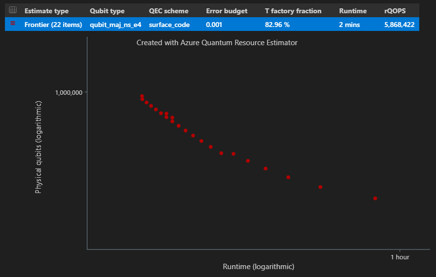
"estimateType"target parameter opgeven als"frontier". Voer bijvoorbeeld hetzelfde algoritme uit met de op Majorana gebaseerde qubitparameters met een surface-code met behulp van pareto grensraming.result = qsharp.estimate("RunProgram()", params= {"qubitParams": { "name": "qubit_maj_ns_e4" }, "qecScheme": { "name": "surface_code" }, "estimateType": "frontier", # frontier estimation } )U kunt de
EstimatesOverviewfunctie gebruiken om een tabel weer te geven met het totale aantal fysieke resources. Klik op het pictogram naast de eerste rij om de kolommen te selecteren die u wilt weergeven. U kunt kiezen uit de uitvoeringsnaam, het schattingstype, het qubittype, het qec-schema, het foutbudget, logische qubits, logische diepte, codeafstand, T-statussen, T-factory's, T factory-breuk, runtime, rQOPS en fysieke qubits.from qsharp_widgets import EstimatesOverview EstimatesOverview(result)
In de kolom Schattingstype van de resultatentabel ziet u het aantal verschillende combinaties van {aantal qubits, runtime} voor uw algoritme. In dit geval vindt de resource-estimator 22 verschillende optimale combinaties van vele duizenden mogelijke combinaties.
Diagram met ruimtetijd
De EstimatesOverview functie geeft ook het ruimte-tijddiagram van de resource-estimator weer.
In het diagram met ruimtetijd ziet u het aantal fysieke qubits en de runtime van het algoritme voor elk {aantal qubits, runtime}-paar. U kunt de muisaanwijzer op elk punt bewegen om de details van de schatting van de resource op dat moment weer te geven.
Batchverwerking met pareto grensraming
Als u meerdere configuraties van target parameters met grensraming wilt schatten en vergelijken, voegt u deze toe
"estimateType": "frontier",aan de parameters.result = qsharp.estimate( "RunProgram()", [ { "qubitParams": { "name": "qubit_maj_ns_e4" }, "qecScheme": { "name": "surface_code" }, "estimateType": "frontier", # Pareto frontier estimation }, { "qubitParams": { "name": "qubit_maj_ns_e6" }, "qecScheme": { "name": "floquet_code" }, "estimateType": "frontier", # Pareto frontier estimation }, ] ) EstimatesOverview(result, colors=["#1f77b4", "#ff7f0e"], runNames=["e4 Surface Code", "e6 Floquet Code"])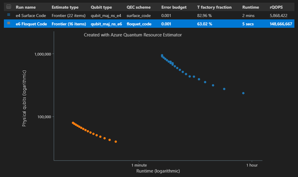
Notitie
U kunt kleuren definiëren en namen uitvoeren voor het qubit-tijddiagram met behulp van de
EstimatesOverviewfunctie.Wanneer u meerdere configuraties van parameters uitvoert met behulp van target de pareto grensraming, kunt u de resourceramingen voor een specifiek punt van het tijddiagram zien, dat voor elk {aantal qubits, runtime}-paar is. In de volgende code ziet u bijvoorbeeld het gebruik van schattingsgegevens voor de tweede uitvoering (schattingsindex=0) en de vierde (puntindex=3) kortste runtime.
EstimateDetails(result[1], 4)U kunt ook het ruimtediagram voor een specifiek punt van het ruimtetijddiagram zien. De volgende code toont bijvoorbeeld het ruimtediagram voor de eerste uitvoering van combinaties (schatting van index=0) en de derde kortste runtime (puntindex=2).
SpaceChart(result[0], 2)
Vereisten voor Qiskit in VS Code
Een Python-omgeving waarop Python en Pip zijn geïnstalleerd.
De nieuwste versie van Visual Studio Code of open Visual Studio Code in de browser.
VS Code met de Quantum Development Kit, Pythonen Jupyter-extensies geïnstalleerd.
De nieuwste Azure Quantum
qsharp- enqsharp_widgets- enqiskit-pakketten.python -m pip install --upgrade qsharp qsharp_widgets qiskitof
!pip install --upgrade qsharp qsharp_widgets qiskit
Tip
U hoeft geen Azure-account te hebben om de resource-estimator uit te voeren.
Een nieuw Jupyter-notebook maken
- Selecteer in VS Code het > Weergeven en selecteer Maken: Nieuw Jupyter Notebook.
- In de rechterbovenhoek detecteert en geeft VS Code de versie van Python en de virtuele Python-omgeving weer die is geselecteerd voor het notebook. Als u meerdere Python-omgevingen hebt, moet u mogelijk een kernel selecteren met behulp van de kernelkiezer in de rechterbovenhoek. Als er geen omgeving is gedetecteerd, raadpleegt u Jupyter Notebooks in VS Code voor informatie over de installatie.
Het kwantumalgoritmen maken
In dit voorbeeld maakt u een kwantumcircuit voor een vermenigvuldiger op basis van de constructie die wordt gepresenteerd in Den Haag-Perez en Garcia-Escartin (arXiv:1411.5949) die gebruikmaakt van de Quantum Fourier Transform om rekenkundige bewerkingen te implementeren.
U kunt de grootte van de vermenigvuldiger aanpassen door de bitwidth variabele te wijzigen. Het genereren van het circuit wordt verpakt in een functie die kan worden aangeroepen met de bitwidth waarde van de vermenigvuldiger. De bewerking heeft twee invoerregisters, elke grootte van de opgegeven bitwidth, en één uitvoerregister die twee keer de grootte van de opgegeven bitwidthis . Met de functie worden ook enkele logische resourceaantallen afgedrukt voor de vermenigvuldiger die rechtstreeks uit het kwantumcircuit is geëxtraheerd.
from qiskit.circuit.library import RGQFTMultiplier

def create_algorithm(bitwidth):
    print(f"[INFO] Create a QFT-based multiplier with bitwidth {bitwidth}")

    circ = RGQFTMultiplier(num_state_qubits=bitwidth)

    return circ
Notitie
Als u een Python-kernel selecteert en de qiskit module niet wordt herkend, selecteert u een andere Python-omgeving in de kernelkiezer.
Het kwantumalgoritmen schatten
Maak een exemplaar van uw algoritme met behulp van de create_algorithm functie. U kunt de grootte van de vermenigvuldiger aanpassen door de bitwidth variabele te wijzigen.
bitwidth = 4

circ = create_algorithm(bitwidth)
Maak een schatting van de fysieke resources voor deze bewerking met behulp van de standaardveronderstellingen. U kunt de estimate-aanroep gebruiken, die overbelast is om een QuantumCircuit-object van Qiskit te accepteren.
from qsharp.estimator import EstimatorParams
from qsharp.interop.qiskit import estimate

params = EstimatorParams()
result = estimate(circ, params)
U kunt ook de ResourceEstimatorBackend gebruiken om de schatting uit te voeren zoals de bestaande back-end dat doet.
from qsharp.interop.qiskit import ResourceEstimatorBackend
from qsharp.estimator import EstimatorParams

params = EstimatorParams()
backend = ResourceEstimatorBackend()

job = backend.run(circ, params)
result = job.result()
Het result-object bevat de uitvoer van de resource-schattingstaak. U kunt de functie EstimateDetails gebruiken om de resultaten weer te geven in een beter leesbare indeling.
from qsharp_widgets import EstimateDetails
EstimateDetails(result)
EstimateDetails functie geeft een tabel weer met het totale aantal fysieke resources. U kunt kostendetails inspecteren door de groepen uit te vouwen, die meer informatie hebben. Zie de volledige rapportgegevens van de resource-estimator voor meer informatie.
Als u bijvoorbeeld de Logische qubitparameters groep uitvouwt, kunt u gemakkelijker zien dat de foutcorrectiecode-afstand 15 is.
| Parameter logische qubit | Weergegeven als |
|---|---|
| QEC-schema | surface_code |
| Codeafstand | 15 |
| Fysieke qubits | 450 |
| Tijd van logische cyclus | 6us |
| Foutpercentage logische qubit | 3.00E-10 |
| Kruising vooraf | 0.03 |
| Drempelwaarde voor foutcorrectie | 0,01 |
| Formule voor tijd van logische cyclus | (4 * twoQubitGateTime + 2 * oneQubitMeasurementTime) * * codeDistance |
| Formule voor fysieke qubits | 2 * codeDistance * codeDistance |
In de groep parameters voor fysieke qubits kunt u de eigenschappen van de fysieke qubit zien die zijn aangenomen voor deze schatting. De tijd voor het uitvoeren van een meting met één qubit en een poort met één qubit wordt bijvoorbeeld uitgegaan van respectievelijk 100 ns en 50 ns.
Tip
U kunt ook toegang krijgen tot de uitvoer van de resource-estimator als een Python-woordenlijst met behulp van de methode result.data(). Als u bijvoorbeeld toegang wilt verkrijgen tot de fysieke tellingen result.data()["physicalCounts"].
Ruimtediagrammen
De verdeling van fysieke qubits die worden gebruikt voor het algoritme en de T-factory's is een factor die van invloed kan zijn op het ontwerp van uw algoritme. U kunt deze distributie visualiseren om meer inzicht te krijgen in de geschatte ruimtevereisten voor het algoritme.
from qsharp_widgets import SpaceChart

SpaceChart(result)
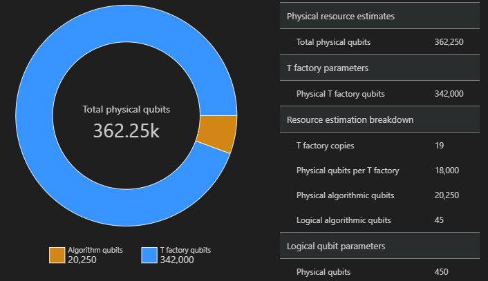
In het ruimtediagram ziet u het aandeel van algoritme-qubits en T Factory-qubits. Houd er rekening mee dat het aantal T-fabriekkopieën, 19, bijdraagt aan het aantal fysieke qubits voor T-fabrieken als $\text{T-fabrieken} \cdot \text{fysieke qubits per T-fabriek} = 19 \cdot 18.000 = 342.000$.
Zie de fysieke schatting van T Factory voor meer informatie.
De standaardwaarden wijzigen en het algoritme schatten
Wanneer u een aanvraag voor een resourceraming voor uw programma indient, kunt u enkele optionele parameters opgeven. Gebruik het jobParams veld om toegang te krijgen tot alle waarden die kunnen worden doorgegeven aan de taakuitvoering en om te zien welke standaardwaarden zijn aangenomen:
result.data()["jobParams"]
{'errorBudget': 0.001,
 'qecScheme': {'crossingPrefactor': 0.03,
  'errorCorrectionThreshold': 0.01,
  'logicalCycleTime': '(4 * twoQubitGateTime + 2 * oneQubitMeasurementTime) * codeDistance',
  'name': 'surface_code',
  'physicalQubitsPerLogicalQubit': '2 * codeDistance * codeDistance'},
 'qubitParams': {'instructionSet': 'GateBased',
  'name': 'qubit_gate_ns_e3',
  'oneQubitGateErrorRate': 0.001,
  'oneQubitGateTime': '50 ns',
  'oneQubitMeasurementErrorRate': 0.001,
  'oneQubitMeasurementTime': '100 ns',
  'tGateErrorRate': 0.001,
  'tGateTime': '50 ns',
  'twoQubitGateErrorRate': 0.001,
  'twoQubitGateTime': '50 ns'}}
Dit zijn de target parameters die kunnen worden aangepast:
-
errorBudget- het totale toegestane foutbudget -
qecScheme- het QEC-schema (kwantumfoutcorrectie) -
qubitParams- de parameters van de fysieke qubit -
constraints- de beperkingen op onderdeelniveau -
distillationUnitSpecifications- de specificaties voor T factory's destillatiealgoritmen
Zie Target de parameters voor de resource-estimator voor meer informatie.
Qubitmodel wijzigen
Maak vervolgens een schatting van de kosten voor hetzelfde algoritme met behulp van de op Majorana gebaseerde qubitparameter qubit_maj_ns_e6
qubitParams = {
    "name": "qubit_maj_ns_e6"
}

result = backend.run(circ, qubitParams).result()
U kunt de fysieke tellingen programmatisch inspecteren. U kunt bijvoorbeeld details verkennen over de T-factory die is gemaakt om het algoritme uit te voeren.
result.data()["tfactory"]
{'eccDistancePerRound': [1, 1, 5],
 'logicalErrorRate': 1.6833177305222897e-10,
 'moduleNamePerRound': ['15-to-1 space efficient physical',
  '15-to-1 RM prep physical',
  '15-to-1 RM prep logical'],
 'numInputTstates': 20520,
 'numModulesPerRound': [1368, 20, 1],
 'numRounds': 3,
 'numTstates': 1,
 'physicalQubits': 16416,
 'physicalQubitsPerRound': [12, 31, 1550],
 'runtime': 116900.0,
 'runtimePerRound': [4500.0, 2400.0, 110000.0]}
Notitie
Runtime wordt standaard weergegeven in nanoseconden.
U kunt deze gegevens gebruiken om enkele uitleg te geven over hoe de T-fabrieken de vereiste T-statussen produceren.
data = result.data()
tfactory = data["tfactory"]
breakdown = data["physicalCounts"]["breakdown"]
producedTstates = breakdown["numTfactories"] * breakdown["numTfactoryRuns"] * tfactory["numTstates"]

print(f"""A single T factory produces {tfactory["logicalErrorRate"]:.2e} T states with an error rate of (required T state error rate is {breakdown["requiredLogicalTstateErrorRate"]:.2e}).""")
print(f"""{breakdown["numTfactories"]} copie(s) of a T factory are executed {breakdown["numTfactoryRuns"]} time(s) to produce {producedTstates} T states ({breakdown["numTstates"]} are required by the algorithm).""")
print(f"""A single T factory is composed of {tfactory["numRounds"]} rounds of distillation:""")
for round in range(tfactory["numRounds"]):
    print(f"""- {tfactory["numUnitsPerRound"][round]} {tfactory["unitNamePerRound"][round]} unit(s)""")
A single T factory produces 1.68e-10 T states with an error rate of (required T state error rate is 2.77e-08).
23 copies of a T factory are executed 523 time(s) to produce 12029 T states (12017 are required by the algorithm).
A single T factory is composed of 3 rounds of distillation:
- 1368 15-to-1 space efficient physical unit(s)
- 20 15-to-1 RM prep physical unit(s)
- 1 15-to-1 RM prep logical unit(s)
Kwantumfoutcorrectieschema wijzigen
Voer nu de resourceramingstaak opnieuw uit voor hetzelfde voorbeeld op de qubitparameters op basis van Majorana met een ge floqued QEC-schema. qecScheme
params = {
    "qubitParams": {"name": "qubit_maj_ns_e6"},
    "qecScheme": {"name": "floquet_code"}
}

result_maj_floquet = backend.run(circ, params).result()
EstimateDetails(result_maj_floquet)
Foutbudget wijzigen
Laten we hetzelfde kwantumcircuit opnieuw uitvoeren met een errorBudget van 10%.
params = {
    "errorBudget": 0.01,
    "qubitParams": {"name": "qubit_maj_ns_e6"},
    "qecScheme": {"name": "floquet_code"},
}
result_maj_floquet_e1 = backend.run(circ, params).result()
EstimateDetails(result_maj_floquet_e1)
Notitie
Als er een probleem optreedt tijdens het werken met de resource-estimator, bekijkt u de pagina Probleemoplossing of neemt u contact op AzureQuantumInfo@microsoft.com.