Design forecast models

Forecast models let you arrange and configure steps to define the forecast that a forecast profile makes. Each model presents a flowchart that graphically represents the calculation that the model does.

For a presentation about how forecast models and outlier removal methods work in Demand planning, watch the following video on YouTube (starting at 16:53): Deep dive into Demand Planning for Supply Chain Management | Dynamics 365 TechTalk.

Create and customize a forecast model

To create and customize a forecast model, you must first open an existing forecast profile. (Learn more in Work with forecast profiles.) You can then fully customize the model that the selected profile uses by adding, removing, and arranging steps, and configuring settings for each of them.

Follow these steps to create and customize a forecast model.

1. On the navigation pane, select Operations > Forecast profiles.
2. Select the forecast profile that you want to create or customize a forecast model for.
3. On the Forecast model tab, there is always at least one step of the Input type at the top of the flow chart. The model is processed from top to bottom, and the last step must be a step of the Save type. Add, remove, and arrange steps as you require, and configure settings for each of them. The illustration after this procedure provides guidelines.
4. After you finish designing your forecast model, select the Validate button in the upper-right corner. The system runs a few tests to validate that your model will work, and then provides feedback. Fix any issues that the validation test reports.
5. Continue to work until your model is ready. Then, on the Action Pane, select Save.
6. If you want to save your forecast model as a preset, so that it's available when you and other users create a new forecast profile, select the Save as model template button in the upper-right corner.

The following illustration shows the information and controls that are available for steps in a forecast model.

Legend:

1. Step symbol – A representation of the purpose of the step.

2. Step type – The type of step. This text usually describes the type of roles, calculations, or other actions that the step represents.

3. Step name – The name that is applied to the step. Sometimes, you can manually enter this text in the step's settings. However, it usually indicates the value of one of the settings that were configured for the step.

4. Step actions – Open a menu of actions that you can take on the step. Although some of these actions are specific to the step type, most are common to all steps. If any actions appear dimmed, they can't be used because of the step's current position or for some other contextual reason. Here are some common actions that are available:

   • Settings – Open a dialog box where you can configure settings for the step.
   • Remove – Remove the step.
   • Move Up and Move Down – Reposition the step in the flowchart.
   • Set to 'Pass Through' – Temporarily disable a currently enabled step without deleting it or its settings.
   • Unset 'Pass Through' – Reenable a currently disabled step.
   • Connect with – For steps that support multiple inputs, specify the second input. The first input is automatically set based on where you put the step.

5. Add a step – Add a new step at the selected location.

Forecast step types

This section describes the purpose of each type of forecast step. It also explains how to use and configure each type.

Input steps

Input steps represent a time series that provides input to the forecast model. All forecast models must start with an Input step.

Settings for Input steps

Input steps have the following settings:

• Step name – The specific name of the step. This name automatically matches the name of the time series.
• Description – A short description of the step.
• Created by – The user who created the step.
• Time series – The time series that is added by the step. When you first set up an Input step, the Configure step dialog box provides a button that lets you select the time series to add. After you add a time series, the dialog box shows the name of the time series and provides an Edit button that lets you change the time series. It also provides a Filter button that lets you set up filtering criteria based on fixed dates, relative dates, and/or field values.
• Time series version – If the selected time series includes more than one version, you can select a specific version. By default, the latest (current) version is used.
• Fill missing values – Specify whether the system should fill in placeholder values for time buckets if the input doesn't provide values. In most cases, you should enable this feature, because it helps produce better forecasts.
• Fill missing values strategy – Select the strategy that the system should use to enter values in empty time buckets. In the current version, the only available strategy is Zeros. In this strategy, the system sets all missing values to 0 (zero).

Signal steps (preview)

[This section is prerelease documentation and is subject to change.]

Signal steps represent additional time series that can be combined with the primary time series that the Input step provides. For example, the primary input that the Input step provides might represent historical sales. A Signal step might then provide input that represents inflation or weather data.

When you add a Signal step, the system automatically creates a parallel branch in your model and puts the step at the top of that branch. The initial branch always has an Input step at the top of it. Each branch can include any number of steps, but you must eventually combine the branches by using a Forecast with signals step.

Settings for Signal steps

Signal steps have the following settings:

• Step name – The specific name of the step. This name automatically matches the name of the time series.
• Description – A short description of the step.
• Created by – The user who created the step.
• Time series – The time series that is added by the step. When you first set up a Signal step, the Configure step dialog box provides a button that lets you select the time series to add. After you add a time series, the dialog box shows the name of the time series and provides an Edit button that lets you change the time series. It also provides a Filter button that lets you set up filtering criteria based on fixed dates, relative dates, and/or field values.
• Time series version – If the selected time series includes more than one version, you can select a specific version. By default, the latest (current) version is used.
• Fill missing values – Specify whether the system should fill in placeholder values for time buckets if the input doesn't provide values. In most cases, you should enable this feature, because it helps produce better forecasts. In the current version, all missing values are set to 0 (zero).

Important

• This is a preview feature.
• Preview features aren’t meant for production use and might have restricted functionality. These features are subject to supplemental terms of use, and are available before an official release so that customers can get early access and provide feedback.

Handle outliers steps

Handle outliers steps identify and compensate for outlier data points in the input. These data points are considered anomalies that should be ignored or smoothed out to prevent them from throwing off the forecast calculation.

Settings for Handle outlier steps

Handle outliers steps have the following settings:

• Step name – The specific name of the step. This name is also shown in the flowchart.

• Description – A short description of the step.

• Created by – The user who created the step.

• Handle outliers – Select one of the following options. Learn more about these options in the How the handle outliers options work section.

  • Interquartile range (IQR)
  • Seasonal and trend decomposition using Loess (STL)

• Interquartile range multiplier – This field is available only when the Handle outliers field is set to IQR. It affects the number of data points that are removed as outliers. Learn more about this setting in the How the handle outliers options work section.

• Correction methods – This field is available only when the Handle outliers field is set to IQR. It affects how outliers are replaced in the data after they are removed. The available options are Median smoothing and Mean smoothing.

• Seasonality hint – This field is available only when the Handle outliers field is set to STL. It influences the size of the window that is used for locally estimated scatterplot smoothing (LOESS) when the seasonal component is estimated. Learn more about this setting in the Seasonality in forecasts section.

How to choose the method for handling outliers

The following table provides examples that will help you choose which method to use to handle outliers in your time series data, based on your scenario.

Scenario	IQR	STL
Data with seasonal or trend patterns	Not recommended	Recommended
Robust handling of outliers	Recommended	Not recommended
Sensitivity to extreme values	Recommended	Recommended

How the handle outliers options work

Interquartile range

The interquartile range (IQR) is the range between the first quartile (Q1) and the third quartile (Q3). It measures the spread of the middle 50% of the data. Any data outside the IQR is identified as an outlier that should be smoothed out later. The IQR method applies the following formula to identify outliers:

IQR = Q3 − Q1

Key:

• Q1 – A representation of the twenty-fifth percentile (that is, the value that 25% of the data lies below).
• Q3 – A representation of the seventy-fifth percentile (that is, the value that 75% of the data lies below).

When you use the IQR method to handle outliers, you must set an Interquartile range multiplier value. This value affects the number of data points that are removed as outliers. It's calculated in the following way:

• Lower bound = Q1 − (Multiplier × IQR​)
• Upper bound = Q3 + (Multiplier × IQR)

A high multiplier increases the range within which data points are considered non-outliers. High multipliers lead to softer boundaries and include more points. Therefore, the result is less sensitive to variations in the time series.

A low multiplier decreases the range within which data points are considered non-outliers. Low multipliers lead to stricter boundaries and remove more data points. Therefore, the result is more sensitive to variations in the time series.

When you use the IQR method to handle outliers, you must also set a Correction method value. This value affects how outliers are replaced in the data after they are removed. The available options are Median smoothing and Mean smoothing.

Seasonal and trend decomposition using LOESS

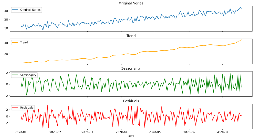
Seasonal and trend decomposition using LOESS (STL) starts by decomposing the time series into three components:

• Trend – The overall trend in the data.
• Seasonality – Regular and predictable patterns that are driven by factors such as weather, holidays, or economic cycles.
• Residuals – The time series after trend and seasonality are removed.

The following illustration shows examples of an original time series, the trend that is decomposed from the time series, the seasonality spikes that are found in the time series, and the residuals after the trend and seasonality are removed.

After STL decomposes the time series, it tries to smooth out the outliers by using LOESS. LOESS is a generalization of the moving average and polynomial regression. It tries to fit a chart through scattered data points and therefore smooth out the residuals, as shown in the following illustration.

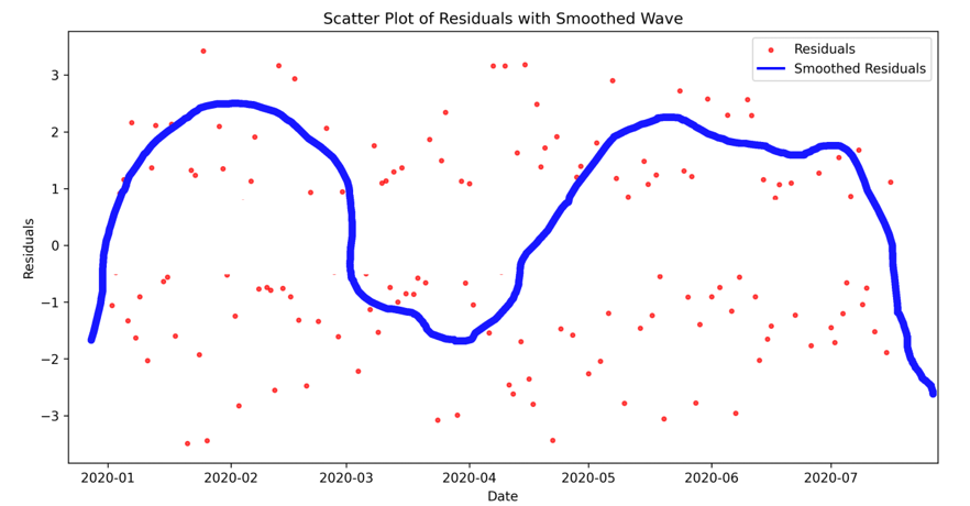
After STL calculates the mean and standard deviation, it uses them to eliminate the outliers and mitigate anomalies.

Finally, STL reintroduces the seasonality and trend to the newly smoothed residual.

When you use the STL method to handle outliers, you must also set a Seasonality hint value. This value influences the size of the period (in time buckets) that is used when the seasonality component is estimated. It helps divide the data into segments to ensure that the algorithm correctly extracts repeating patterns. For example, if you notice a weekly seasonality pattern where most customers shop on Saturdays, and you're using buckets in days, enter 7 as the Seasonality hint value. Learn more about seasonality and seasonality hints in the Seasonality in forecasts section.

Forecast steps

Forecast steps apply a selected forecast algorithm to the input time series to create a forecast time series.

Settings for Forecast steps

Forecast steps have the following settings:

• Step name – The specific name of the step. This name is also shown in the flowchart.

• Description – A short description of the step.

• Created by – The user who created the step.

• Model type – Select the forecast algorithm to use. Learn about each of the available algorithms in Demand forecasting algorithms.

  • Best fit model
  • ARIMA (auto regressive integrated moving average)
  • ETS (error, trend, seasonality)
  • Prophet

• Seasonality hint (in periods of time buckets) – Seasonality refers to a pattern of demand that fluctuates according to a regular, recurring schedule. If your data has such a pattern, enter the frequency (in time buckets). For example, if you notice a weekly seasonality pattern where most customers shop on Saturdays, and you're using buckets in days, enter 7 here. Learn more about seasonality and seasonality hints in the Seasonality in forecasts section.

Forecast with signals (preview)

[This section is prerelease documentation and is subject to change.]

Forecast with signals steps generate a forecast based on two input time series. They always use the XGBoost demand forecasting algorithm. Learn about this algorithm in Demand forecasting algorithms.

You can use this type of step only if your forecast model has at least two parallel branches: one that starts with an Input step and one that starts with a Signal step. The first branch is the one where you create the step. To specify the second branch, open the Action menu for the Forecast with signals step, select Connect with, and then select the step to connect to. The flowchart is then updated so that it shows the two branches combining at the Forecast with signals step.

Settings for Forecast with signals steps

Forecast with signals steps have the following settings:

• Step name – The specific name of the step. This name is also shown in the flowchart.
• Description – A short description of the step.
• Created by – The user who created the step.
• Model type – Select the forecast algorithm to use. In the current version, only the XGBoost algorithm is available.
• Seasonality hint (in periods of time buckets) – Seasonality refers to a pattern of demand that fluctuates according to a regular, recurring schedule. If your data has such a pattern, enter the frequency (in time buckets). For example, if you notice a weekly seasonality pattern where most customers shop on Saturdays, and you're using buckets in days, enter 7 here. Learn more about seasonality and seasonality hints in the Seasonality in forecasts section.

Important

• This is a preview feature.
• Preview features aren’t meant for production use and might have restricted functionality. These features are subject to supplemental terms of use, and are available before an official release so that customers can get early access and provide feedback.

Finance and operations – Azure Machine Learning steps

You might already be using your own custom Microsoft Azure Machine Learning algorithms for demand forecasting in Dynamics 365 Supply Chain Management, as described in Demand forecasting overview. In this case, you can continue to use those algorithms while you use Demand planning. Just put a Finance and operations – Azure Machine Learning step in your forecast model instead of a Forecast step.

Learn how to set up Demand planning to connect to and use your Azure Machine Learning algorithms in Use your own custom Azure Machine Learning algorithms in Demand planning.

Phase in/out steps

Phase in/out steps modify the values of a data column in a time series to simulate the gradual process of phasing in a new element or phasing out an old element. For example, a Phase in/out step might simulate the process of phasing in a new product or warehouse. The phase in/out calculation lasts for a specific period and uses values that are drawn from the same time series. (The values come from either the same data column that is being adjusted or another data column that represents a similar element.)

Settings for Phase in/out steps

Phase in/out steps have the following settings:

• Step name – The specific name of the step. This name is also shown in the flowchart.
• Description – A short description of the step.
• Created by – The user who created the step.
• Rule group – The name of the rule group that defines the calculation that the step does.

When you set up your forecast model, the position of the Phase in/out step affects the calculation result.

• To apply the phase in/out calculation to the historical sales numbers, put the Phase in/out step before the Forecast step, as shown on the left side of the following illustration.
• To apply the phase in/out calculation to the forecasted result, put the Phase in/out step after the Forecast step, as shown on the right side of the illustration.

Learn more about phase in/out functionality, including details about how to set up your phase in/out rule groups, in Use phase in/out functionality to simulate planned changes.

Save steps

Save steps save the result of the forecast model as a new or updated series. All forecast models must end with a single Save step.

The forecast time series is saved according to the settings that you configure each time that you run a forecast job. Learn more in Work with forecast profiles.

Seasonality in forecasts

Seasonality refers to regular and predictable patterns in a time series that occur at fixed intervals because of recurring events or influences. These patterns are often driven by factors such as weather, holidays, or economic cycles. Examples include increased retail sales every December because of holiday shopping or higher electricity demand during summer months because of air conditioning.

Demand planning identifies and compensates for seasonality patterns both when it handles outliers (in a Handle outliers step that is set to use STL) and when it generates a forecast (in any forecast step).

How seasonality differs from cycles

Although both seasonality and cycles involve repeating patterns, there are key differences, as summarized in the following table.

Aspect	Seasonality	Cycles
Frequency	Fixed, regular intervals (such as daily, weekly, or yearly)	Variable, often irregular, and influenced by external factors
Duration	Short-term and predictable (such as seasonal sales)	Long-term and unpredictable (such as business cycles)
Cause	Calendar-based events or natural patterns	Economic, social, or structural forces
Examples	Summer travel peaks or holiday shopping trends	Economic recession cycles or stock market booms and busts

Seasonality hints

Some forecast and outlier detection algorithms provide a Seasonality hint setting. This setting influences the size of the period (in time buckets) that is used in the identification of seasonality patterns. It helps divide the data into segments to ensure that the algorithm correctly extracts repeating patterns. For example, if you notice a weekly seasonality pattern where most customers shop on Saturdays, and you're using buckets in days, enter 7 as the Seasonality hint value.

A well-defined seasonal period captures the true periodicity of the data. It enables the algorithm to successfully isolate the seasonality. As a result, the trend and residuals are more interpretable. By contrast, an incorrect seasonal period leads to poor seasonal extraction. As a result, trend and residual components are inaccurate.

If the seasonal period that you use is too short (that is, shorter than the actual cycle), you risk encountering the following issues:

• Missed patterns – Important parts of the seasonal pattern might be excluded, so that seasonality extraction is incomplete.
• Trend contamination – Some seasonal variations might be mistaken for the trend component, so that the trend estimation is distorted.
• Residual issues – Residuals might show unexplained periodicity. This situation indicates that the algorithm failed to capture seasonality correctly.

For example, you use a seasonal period of 6 months for yearly retail sales data. In this case, only part of the yearly cycle is captured. As a result, critical holiday season peaks might be missing.

If the seasonal period that you use is too long (that is, longer than the actual cycle), you risk encountering the following issues:

• Overfitting – Noise or random fluctuations might be falsely interpreted as seasonality.
• Distorted decomposition – Artificially long seasonal cycles might obscure the true trend or residual components.
• Increased complexity – The model might become unnecessarily complex and therefore harder to interpret and validate.

For example, you use a seasonal period of 24 months for data that has an annual cycle. The result is overfitting, where small irregularities in the data are treated as seasonal patterns.

Autodetect seasonality patterns (preview)

[This section is prerelease documentation and is subject to change.]

If you're using the ARIMA forecast algorithm, the Seasonality hint (in periods of time buckets) setting is replaced by the Select seasonality detection setting (preview) setting. This setting provides the following options:

• Auto detection – Select this option to enable an algorithm that automatically detects seasonality patterns for each combination of a location and a product, and applies the result to forecast calculations. Seasonality patterns typically vary for different products and different locations. Therefore, auto detection often works better than application of the same pattern everywhere.
• Detection using hint – Select this option to use the value that you enter in the Seasonality hint (in periods of time buckets) field to help identify seasonality patterns. This option works best when you know the seasonality pattern in advance. For example, if you know that you have a strong weekly seasonality pattern where most customers shop on Saturdays, and you're using buckets in days, select this option, and then enter 7 in the Seasonality hint (in periods of time buckets) field. Learn more about this setting in the previous section.

Important

• This is a preview feature.
• Preview features aren’t meant for production use and might have restricted functionality. These features are subject to supplemental terms of use, and are available before an official release so that customers can get early access and provide feedback.