使用 PyTorch 训练数据分析模型

在本教程的前一阶段中，我们获取了将用于使用 PyTorch 训练数据分析模型的数据集。 现在，我们将使用这些数据。

要使用 PyTorch 训练数据分析模型，需要完成以下步骤：

1. 加载数据。 如果已完成本教程的上一步，则已经完成了数据加载。
2. 定义神经网络。
3. 定义损失函数。
4. 使用训练数据训练模型。
5. 使用测试数据测试网络。

定义神经网络

在本教程中，你将构建带有 3 个线性层的基本神经网络模型。 模型的结构如下所示：

Linear -> ReLU -> Linear -> ReLU -> Linear

一个线性层对传入数据应用一个线性转换。 必须指定输入特征的数量和输出特征的数量，它们应与类的数量相对应。

ReLU 层是一个激活函数，用于将所有传入特征定义为 0 或更大。 因此，应用此层时，任何小于 0 的数字都会更改为零，而其他数字则保持不变。 我们将在 2 个隐藏层上应用激活层，在最后一个线性层上不应用激活层。

模型参数

模型参数取决于我们的目标和训练数据。 输入大小取决于我们向模型馈送的特征数量，在本例中为 4 个。 输出大小是 3，因为有 3 种可能的鸢尾花类型。

有 3 个线性层 (4,24) -> (24,24) -> (24,3)，网络将具有 744 个权重 (96+576+72)。

学习速率 (lr) 设置你根据损失梯度调整网络权重的程度控制。 速率越低，训练速度就越慢。 你将在本教程中将 lr 设置为 0.01。

网络是如何运作的？

在此处，我们将构建一个前馈网络。 在训练过程中，网络将处理所有层的输入，计算损失以了解图像的预测标签与正确标签相差多远，并将梯度传播回网络以更新层的权重。 通过迭代庞大的输入数据集，网络将“学习”设置其权重以获得最佳结果。

前向函数计算损失函数的值，后向函数计算可学习参数的梯度。 使用 PyTorch 创建神经网络时，只需定义前向函数。 后向函数会自动定义。

1. 将以下代码复制到 Visual Studio 中的 DataClassifier.py 文件中，来定义模型参数和神经网络。

# Define model parameters 
input_size = list(input.shape)[1]   # = 4. The input depends on how many features we initially feed the model. In our case, there are 4 features for every predict value  
learning_rate = 0.01 
output_size = len(labels)           # The output is prediction results for three types of Irises.  


# Define neural network 
class Network(nn.Module): 
   def __init__(self, input_size, output_size): 
       super(Network, self).__init__() 
        
       self.layer1 = nn.Linear(input_size, 24) 
       self.layer2 = nn.Linear(24, 24) 
       self.layer3 = nn.Linear(24, output_size) 


   def forward(self, x): 
       x1 = F.relu(self.layer1(x)) 
       x2 = F.relu(self.layer2(x1)) 
       x3 = self.layer3(x2) 
       return x3 
 
# Instantiate the model 
model = Network(input_size, output_size) 

还需要根据电脑上的可用设备来定义执行设备。 PyTorch 没有用于 GPU 的专用库，但你可手动定义执行设备。 如果计算机上存在 Nvidia GPU，则该设备为 Nvidia GPU；如果没有，则为 CPU。

2. 复制以下代码来定义执行设备：

# Define your execution device 
device = torch.device("cuda:0" if torch.cuda.is_available() else "cpu") 
print("The model will be running on", device, "device\n") 
model.to(device)    # Convert model parameters and buffers to CPU or Cuda 

3. 最后一步是定义函数来保存模型：

# Function to save the model 
def saveModel(): 
    path = "./NetModel.pth" 
    torch.save(model.state_dict(), path) 

注意

想要详细了解如何使用 PyTorch 创建神经网络？ 请查看 PyTorch 文档。

定义损失函数

损失函数计算一个值，该值可估计输出与目标之间的差距。 主要目标是通过神经网络中的反向传播改变权重向量值来减少损失函数的值。

丢失值不同于模型准确性。 损失函数表示模型在每次训练集优化迭代后的表现。 模型的准确性基于测试数据进行计算，并显示正确预测的百分比。

在 PyTorch 中，神经网络包包含各种损失函数，这些函数构成了深层神经网络的构建基块。 若想详细了解这些细节，请先查看上述说明。 在此处，我们将使用针对这种分类优化的现有函数，并使用分类交叉熵损失函数和 Adam 优化器。 在该优化器中，学习速率 (lr) 设置你根据损失梯度调整网络权重的程度控制。 此处需要将它设置为 0.001 - 值越低，训练速度越慢。

1. 将以下代码复制到 Visual Studio 中的 DataClassifier.py 文件中，以定义损失函数和优化器。

# Define the loss function with Classification Cross-Entropy loss and an optimizer with Adam optimizer
loss_fn = nn.CrossEntropyLoss()
optimizer = Adam(model.parameters(), lr=0.001, weight_decay=0.0001)

使用训练数据训练模型。

要训练模型，必须循环访问数据迭代器，将输入馈送到网络并进行优化。 只需在每次训练 epoch 后将预测得到的标签与验证数据集中的实际标签进行比较，即可验证结果。

该程序将显示针对训练集的每个 epoch 或每个完整迭代的训练损失、验证损失和模型准确度。 它将以最高准确度保存模型，在 10 个 epoch 后，程序将显示最终的准确度。

1. 将以下代码添加到 DataClassifier.py 文件

# Training Function 
def train(num_epochs): 
    best_accuracy = 0.0 
     
    print("Begin training...") 
    for epoch in range(1, num_epochs+1): 
        running_train_loss = 0.0 
        running_accuracy = 0.0 
        running_vall_loss = 0.0 
        total = 0 
 
        # Training Loop 
        for data in train_loader: 
        #for data in enumerate(train_loader, 0): 
            inputs, outputs = data  # get the input and real species as outputs; data is a list of [inputs, outputs] 
            optimizer.zero_grad()   # zero the parameter gradients          
            predicted_outputs = model(inputs)   # predict output from the model 
            train_loss = loss_fn(predicted_outputs, outputs)   # calculate loss for the predicted output  
            train_loss.backward()   # backpropagate the loss 
            optimizer.step()        # adjust parameters based on the calculated gradients 
            running_train_loss +=train_loss.item()  # track the loss value 
 
        # Calculate training loss value 
        train_loss_value = running_train_loss/len(train_loader) 
 
        # Validation Loop 
        with torch.no_grad(): 
            model.eval() 
            for data in validate_loader: 
               inputs, outputs = data 
               predicted_outputs = model(inputs) 
               val_loss = loss_fn(predicted_outputs, outputs) 
             
               # The label with the highest value will be our prediction 
               _, predicted = torch.max(predicted_outputs, 1) 
               running_vall_loss += val_loss.item()  
               total += outputs.size(0) 
               running_accuracy += (predicted == outputs).sum().item() 
 
        # Calculate validation loss value 
        val_loss_value = running_vall_loss/len(validate_loader) 
                
        # Calculate accuracy as the number of correct predictions in the validation batch divided by the total number of predictions done.  
        accuracy = (100 * running_accuracy / total)     
 
        # Save the model if the accuracy is the best 
        if accuracy > best_accuracy: 
            saveModel() 
            best_accuracy = accuracy 
         
        # Print the statistics of the epoch 
        print('Completed training batch', epoch, 'Training Loss is: %.4f' %train_loss_value, 'Validation Loss is: %.4f' %val_loss_value, 'Accuracy is %d %%' % (accuracy))

使用测试数据测试模型。

现在我们已经训练了模型，接下来可使用测试数据集来测试模型。

我们将添加 2 个测试函数。 第一个函数测试你在上一部分保存的模型。 它将使用包含 45 个项的测试数据集来测试模型，并打印出模型的准确度。 第二个是可选函数，用于测试模型在预测三种鸢尾花品类的每一种时的可信度，用成功分类每个品种的概率表示。

1. 将以下代码添加到 DataClassifier.py 文件。

# Function to test the model 
def test(): 
    # Load the model that we saved at the end of the training loop 
    model = Network(input_size, output_size) 
    path = "NetModel.pth" 
    model.load_state_dict(torch.load(path)) 
     
    running_accuracy = 0 
    total = 0 
 
    with torch.no_grad(): 
        for data in test_loader: 
            inputs, outputs = data 
            outputs = outputs.to(torch.float32) 
            predicted_outputs = model(inputs) 
            _, predicted = torch.max(predicted_outputs, 1) 
            total += outputs.size(0) 
            running_accuracy += (predicted == outputs).sum().item() 
 
        print('Accuracy of the model based on the test set of', test_split ,'inputs is: %d %%' % (100 * running_accuracy / total))    
 
 
# Optional: Function to test which species were easier to predict  
def test_species(): 
    # Load the model that we saved at the end of the training loop 
    model = Network(input_size, output_size) 
    path = "NetModel.pth" 
    model.load_state_dict(torch.load(path)) 
     
    labels_length = len(labels) # how many labels of Irises we have. = 3 in our database. 
    labels_correct = list(0. for i in range(labels_length)) # list to calculate correct labels [how many correct setosa, how many correct versicolor, how many correct virginica] 
    labels_total = list(0. for i in range(labels_length))   # list to keep the total # of labels per type [total setosa, total versicolor, total virginica] 
  
    with torch.no_grad(): 
        for data in test_loader: 
            inputs, outputs = data 
            predicted_outputs = model(inputs) 
            _, predicted = torch.max(predicted_outputs, 1) 
             
            label_correct_running = (predicted == outputs).squeeze() 
            label = outputs[0] 
            if label_correct_running.item():  
                labels_correct[label] += 1 
            labels_total[label] += 1  
  
    label_list = list(labels.keys()) 
    for i in range(output_size): 
        print('Accuracy to predict %5s : %2d %%' % (label_list[i], 100 * labels_correct[i] / labels_total[i])) 

最后，让我们添加主代码。 这将启动模型训练、保存模型并在屏幕上显示结果。 我们将在训练集上仅运行两次迭代 [num_epochs = 25]，因此训练过程不会花费太长时间。

2. 将以下代码添加到 DataClassifier.py 文件。

if __name__ == "__main__": 
    num_epochs = 10
    train(num_epochs) 
    print('Finished Training\n') 
    test() 
    test_species() 

让我们运行测试！ 确保顶部工具栏中的下拉菜单设置为 Debug。 如果设备是 64 位的，请将 Solution Platform 更改为 x64 以在本地计算机上运行项目；如果设备是 32 位的，请将其更改为 x86。

3. 要运行项目，请单击工具栏上的 Start Debugging 按钮，或者按 F5。

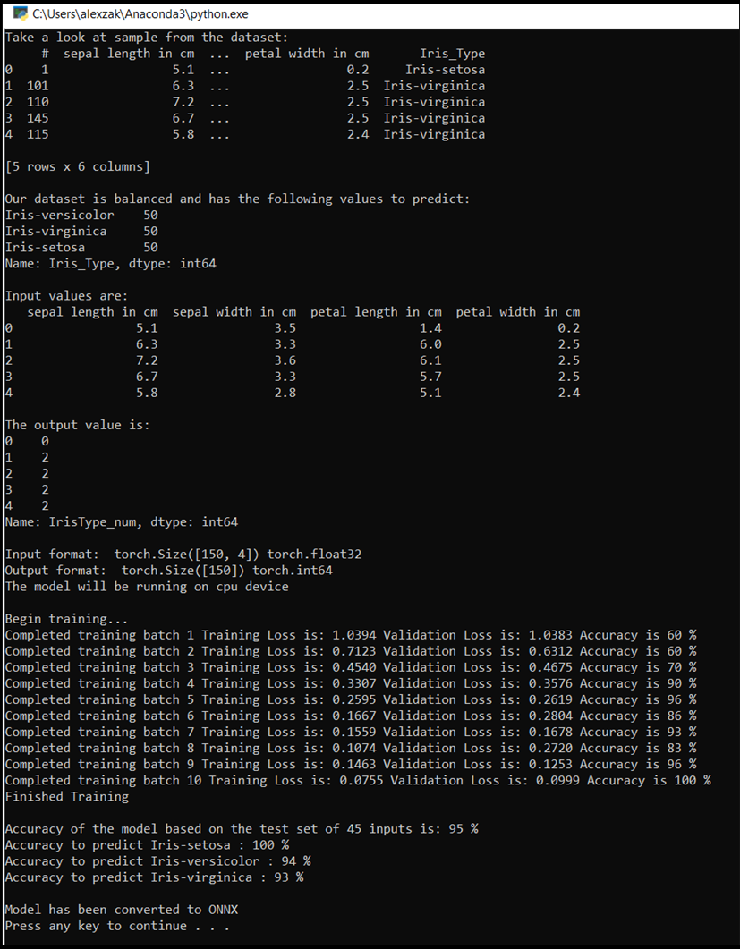
这将弹出控制台窗口，你将看到训练过程。 如定义的一样，将对每个 epoch 打印丢失值。 预期是随着每次 epoch，损失值会变小。

训练完成后，应会看到类似于下面的输出。 数字不会完全相同 - 训练取决于许多因素，并且不会总是返回相同的结果 - 但它们应该看起来相似。

后续步骤

现在我们有了一个分类模型，下一步是将模型转换为 ONNX 格式。