练习 - 估算实际问题的资源

10 分钟

Shor 因子分解算法是最著名的量子算法之一。它可以指数加速任何已知经典因子算法。

经典加密使用物理或数学手段（如计算难度）来完成任务。常用的加密协议是 Rivest-Shamir-Adleman (RSA) 方案，该方案基于使用经典计算机对质数进行因式分解的难度假设。

Shor 算法意味着足够大的量子计算机可以破解公钥加密。估计 Shor 算法所需的资源对于评估这些类型的加密方案的漏洞非常重要。

在以下练习中，你将计算 2,048 位整数的因式分解的资源估算值。对于此应用程序，将直接通过预计算的逻辑资源估算值来计算物理资源估算值。对于容许误差预算，将使用 $\epsilon = 1/3$。

编写 Shor 算法

在 Visual Studio Code 中，选择“视图 > 命令面板”，然后选择“创建：新 Jupyter Notebook”。
将笔记本另存为 ShorRE.ipynb。
在第一个单元格中，导入 qsharp 包：
```
import qsharp
```

使用 Microsoft.Quantum.ResourceEstimation 命名空间定义 Shor 整数分解算法的缓存优化版本。添加新单元格，然后粘贴并复制以下代码：

%%qsharp
open Microsoft.Quantum.Arrays;
open Microsoft.Quantum.Canon;
open Microsoft.Quantum.Convert;
open Microsoft.Quantum.Diagnostics;
open Microsoft.Quantum.Intrinsic;
open Microsoft.Quantum.Math;
open Microsoft.Quantum.Measurement;
open Microsoft.Quantum.Unstable.Arithmetic;
open Microsoft.Quantum.ResourceEstimation;

operation RunProgram() : Unit {
    let bitsize = 31;

    // When choosing parameters for `EstimateFrequency`, make sure that
    // generator and modules are not co-prime
    let _ = EstimateFrequency(11, 2^bitsize - 1, bitsize);
}


// In this sample we concentrate on costing the `EstimateFrequency`
// operation, which is the core quantum operation in Shors algorithm, and
// we omit the classical pre- and post-processing.

/// # Summary
/// Estimates the frequency of a generator
/// in the residue ring Z mod `modulus`.
///
/// # Input
/// ## generator
/// The unsigned integer multiplicative order (period)
/// of which is being estimated. Must be co-prime to `modulus`.
/// ## modulus
/// The modulus which defines the residue ring Z mod `modulus`
/// in which the multiplicative order of `generator` is being estimated.
/// ## bitsize
/// Number of bits needed to represent the modulus.
///
/// # Output
/// The numerator k of dyadic fraction k/2^bitsPrecision
/// approximating s/r.
operation EstimateFrequency(
    generator : Int,
    modulus : Int,
    bitsize : Int
)
: Int {
    mutable frequencyEstimate = 0;
    let bitsPrecision =  2 * bitsize + 1;

    // Allocate qubits for the superposition of eigenstates of
    // the oracle that is used in period finding.
    use eigenstateRegister = Qubit[bitsize];

    // Initialize eigenstateRegister to 1, which is a superposition of
    // the eigenstates we are estimating the phases of.
    // We first interpret the register as encoding an unsigned integer
    // in little endian encoding.
    ApplyXorInPlace(1, eigenstateRegister);
    let oracle = ApplyOrderFindingOracle(generator, modulus, _, _);

    // Use phase estimation with a semiclassical Fourier transform to
    // estimate the frequency.
    use c = Qubit();
    for idx in bitsPrecision - 1..-1..0 {
        within {
            H(c);
        } apply {
            // `BeginEstimateCaching` and `EndEstimateCaching` are the operations
            // exposed by Azure Quantum Resource Estimator. These will instruct
            // resource counting such that the if-block will be executed
            // only once, its resources will be cached, and appended in
            // every other iteration.
            if BeginEstimateCaching("ControlledOracle", SingleVariant()) {
                Controlled oracle([c], (1 <<< idx, eigenstateRegister));
                EndEstimateCaching();
            }
            R1Frac(frequencyEstimate, bitsPrecision - 1 - idx, c);
        }
        if MResetZ(c) == One {
            set frequencyEstimate += 1 <<< (bitsPrecision - 1 - idx);
        }
    }

    // Return all the qubits used for oracles eigenstate back to 0 state
    // using Microsoft.Quantum.Intrinsic.ResetAll.
    ResetAll(eigenstateRegister);

    return frequencyEstimate;
}

/// # Summary
/// Interprets `target` as encoding unsigned little-endian integer k
/// and performs transformation |k⟩ ↦ |gᵖ⋅k mod N ⟩ where
/// p is `power`, g is `generator` and N is `modulus`.
///
/// # Input
/// ## generator
/// The unsigned integer multiplicative order ( period )
/// of which is being estimated. Must be co-prime to `modulus`.
/// ## modulus
/// The modulus which defines the residue ring Z mod `modulus`
/// in which the multiplicative order of `generator` is being estimated.
/// ## power
/// Power of `generator` by which `target` is multiplied.
/// ## target
/// Register interpreted as LittleEndian which is multiplied by
/// given power of the generator. The multiplication is performed modulo
/// `modulus`.
internal operation ApplyOrderFindingOracle(
    generator : Int, modulus : Int, power : Int, target : Qubit[]
)
: Unit
is Adj + Ctl {
    // The oracle we use for order finding implements |x⟩ ↦ |x⋅a mod N⟩. We
    // also use `ExpModI` to compute a by which x must be multiplied. Also
    // note that we interpret target as unsigned integer in little-endian
    // encoding by using the `LittleEndian` type.
    ModularMultiplyByConstant(modulus,
                                ExpModI(generator, power, modulus),
                                target);
}

/// # Summary
/// Performs modular in-place multiplication by a classical constant.
///
/// # Description
/// Given the classical constants `c` and `modulus`, and an input
/// quantum register (as LittleEndian) |𝑦⟩, this operation
/// computes `(c*x) % modulus` into |𝑦⟩.
///
/// # Input
/// ## modulus
/// Modulus to use for modular multiplication
/// ## c
/// Constant by which to multiply |𝑦⟩
/// ## y
/// Quantum register of target
internal operation ModularMultiplyByConstant(modulus : Int, c : Int, y : Qubit[])
: Unit is Adj + Ctl {
    use qs = Qubit[Length(y)];
    for (idx, yq) in Enumerated(y) {
        let shiftedC = (c <<< idx) % modulus;
        Controlled ModularAddConstant([yq], (modulus, shiftedC, qs));
    }
    ApplyToEachCA(SWAP, Zipped(y, qs));
    let invC = InverseModI(c, modulus);
    for (idx, yq) in Enumerated(y) {
        let shiftedC = (invC <<< idx) % modulus;
        Controlled ModularAddConstant([yq], (modulus, modulus - shiftedC, qs));
    }
}

/// # Summary
/// Performs modular in-place addition of a classical constant into a
/// quantum register.
///
/// # Description
/// Given the classical constants `c` and `modulus`, and an input
/// quantum register (as LittleEndian) |𝑦⟩, this operation
/// computes `(x+c) % modulus` into |𝑦⟩.
///
/// # Input
/// ## modulus
/// Modulus to use for modular addition
/// ## c
/// Constant to add to |𝑦⟩
/// ## y
/// Quantum register of target
internal operation ModularAddConstant(modulus : Int, c : Int, y : Qubit[])
: Unit is Adj + Ctl {
    body (...) {
        Controlled ModularAddConstant([], (modulus, c, y));
    }
    controlled (ctrls, ...) {
        // We apply a custom strategy to control this operation instead of
        // letting the compiler create the controlled variant for us in which
        // the `Controlled` functor would be distributed over each operation
        // in the body.
        //
        // Here we can use some scratch memory to save ensure that at most one
        // control qubit is used for costly operations such as `AddConstant`
        // and `CompareGreaterThenOrEqualConstant`.
        if Length(ctrls) >= 2 {
            use control = Qubit();
            within {
                Controlled X(ctrls, control);
            } apply {
                Controlled ModularAddConstant([control], (modulus, c, y));
            }
        } else {
            use carry = Qubit();
            Controlled AddConstant(ctrls, (c, y + [carry]));
            Controlled Adjoint AddConstant(ctrls, (modulus, y + [carry]));
            Controlled AddConstant([carry], (modulus, y));
            Controlled CompareGreaterThanOrEqualConstant(ctrls, (c, y, carry));
        }
    }
}

/// # Summary
/// Performs in-place addition of a constant into a quantum register.
///
/// # Description
/// Given a non-empty quantum register |𝑦⟩ of length 𝑛+1 and a positive
/// constant 𝑐 < 2ⁿ, computes |𝑦 + c⟩ into |𝑦⟩.
///
/// # Input
/// ## c
/// Constant number to add to |𝑦⟩.
/// ## y
/// Quantum register of second summand and target; must not be empty.
internal operation AddConstant(c : Int, y : Qubit[]) : Unit is Adj + Ctl {
    // We are using this version instead of the library version that is based
    // on Fourier angles to show an advantage of sparse simulation in this sample.

    let n = Length(y);
    Fact(n > 0, "Bit width must be at least 1");

    Fact(c >= 0, "constant must not be negative");
    Fact(c < 2 ^ n, $"constant must be smaller than {2L ^ n}");

    if c != 0 {
        // If c has j trailing zeroes than the j least significant bits
        // of y will not be affected by the addition and can therefore be
        // ignored by applying the addition only to the other qubits and
        // shifting c accordingly.
        let j = NTrailingZeroes(c);
        use x = Qubit[n - j];
        within {
            ApplyXorInPlace(c >>> j, x);
        } apply {
            IncByLE(x, y[j...]);
        }
    }
}

/// # Summary
/// Performs greater-than-or-equals comparison to a constant.
///
/// # Description
/// Toggles output qubit `target` if and only if input register `x`
/// is greater than or equal to `c`.
///
/// # Input
/// ## c
/// Constant value for comparison.
/// ## x
/// Quantum register to compare against.
/// ## target
/// Target qubit for comparison result.
///
/// # Reference
/// This construction is described in [Lemma 3, arXiv:2201.10200]
internal operation CompareGreaterThanOrEqualConstant(c : Int, x : Qubit[], target : Qubit)
: Unit is Adj+Ctl {
    let bitWidth = Length(x);

    if c == 0 {
        X(target);
    } elif c >= 2 ^ bitWidth {
        // do nothing
    } elif c == 2 ^ (bitWidth - 1) {
        ApplyLowTCNOT(Tail(x), target);
    } else {
        // normalize constant
        let l = NTrailingZeroes(c);

        let cNormalized = c >>> l;
        let xNormalized = x[l...];
        let bitWidthNormalized = Length(xNormalized);
        let gates = Rest(IntAsBoolArray(cNormalized, bitWidthNormalized));

        use qs = Qubit[bitWidthNormalized - 1];
        let cs1 = [Head(xNormalized)] + Most(qs);
        let cs2 = Rest(xNormalized);

        within {
            for i in IndexRange(gates) {
                (gates[i] ? ApplyAnd | ApplyOr)(cs1[i], cs2[i], qs[i]);
            }
        } apply {
            ApplyLowTCNOT(Tail(qs), target);
        }
    }
}

/// # Summary
/// Internal operation used in the implementation of GreaterThanOrEqualConstant.
internal operation ApplyOr(control1 : Qubit, control2 : Qubit, target : Qubit) : Unit is Adj {
    within {
        ApplyToEachA(X, [control1, control2]);
    } apply {
        ApplyAnd(control1, control2, target);
        X(target);
    }
}

internal operation ApplyAnd(control1 : Qubit, control2 : Qubit, target : Qubit)
: Unit is Adj {
    body (...) {
        CCNOT(control1, control2, target);
    }
    adjoint (...) {
        H(target);
        if (M(target) == One) {
            X(target);
            CZ(control1, control2);
        }
    }
}


/// # Summary
/// Returns the number of trailing zeroes of a number
///
/// ## Example
/// ```qsharp
/// let zeroes = NTrailingZeroes(21); // = NTrailingZeroes(0b1101) = 0
/// let zeroes = NTrailingZeroes(20); // = NTrailingZeroes(0b1100) = 2
/// ```
internal function NTrailingZeroes(number : Int) : Int {
    mutable nZeroes = 0;
    mutable copy = number;
    while (copy % 2 == 0) {
        set nZeroes += 1;
        set copy /= 2;
    }
    return nZeroes;
}

/// # Summary
/// An implementation for `CNOT` that when controlled using a single control uses
/// a helper qubit and uses `ApplyAnd` to reduce the T-count to 4 instead of 7.
internal operation ApplyLowTCNOT(a : Qubit, b : Qubit) : Unit is Adj+Ctl {
    body (...) {
        CNOT(a, b);
    }

    adjoint self;

    controlled (ctls, ...) {
        // In this application this operation is used in a way that
        // it is controlled by at most one qubit.
        Fact(Length(ctls) <= 1, "At most one control line allowed");

        if IsEmpty(ctls) {
            CNOT(a, b);
        } else {
            use q = Qubit();
            within {
                ApplyAnd(Head(ctls), a, q);
            } apply {
                CNOT(q, b);
            }
        }
    }

    controlled adjoint self;
}

估算 Shor 算法

现在使用默认假设来估算 RunProgram 操作的物理资源。添加新单元格，然后粘贴并复制以下代码：

result = qsharp.estimate("RunProgram()")
result

qsharp.estimate 函数创建一个结果对象，可用于显示整体物理资源计数的表。可以通过折叠包含更多信息的组来检查成本详细信息。

例如，折叠“逻辑量子比特参数”组以查看代码距离为 21，物理量子比特数为 882。

逻辑量子比特参数	值
QEC 方案	surface_code
码距	21
物理量子比特	882
逻辑周期时间	8 毫秒
逻辑量子比特错误率	3.00E-13
交叉预制	0.03
错误更正阈值	0.01
逻辑周期时间公式	(4 * `twoQubitGateTime` + 2 * `oneQubitMeasurementTime`) * `codeDistance`
物理量子比特公式	2 * `codeDistance` * `codeDistance`

提示

对于更紧凑的输出表，可以使用 result.summary。

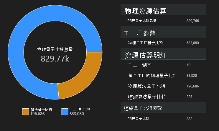
空间图

用于算法和 T 工厂的物理量子比特的分布可能会影响算法的设计。可以使用 qsharp-widgets 包来可视化此分布，以便更好地了解算法的预计空间要求。

from qsharp_widgets import SpaceChart
SpaceChart(result)

在此示例中，运行算法所需的物理量子比特数为 829766，其中 196686 个是算法量子比特，633080 个是 T 工厂量子比特。

显示资源估算器空间图的屏幕截图。

比较不同量子比特技术的资源估算值

使用 Azure Quantum 资源估算器可以运行目标参数的多个配置并比较结果。如果要比较不同量子比特模型、QEC 方案或错误预算的成本，这会非常有用。

还可以使用 EstimatorParams 对象构建估算参数的列表。

from qsharp.estimator import EstimatorParams, QubitParams, QECScheme, LogicalCounts

labels = ["Gate-based µs, 10⁻³", "Gate-based µs, 10⁻⁴", "Gate-based ns, 10⁻³", "Gate-based ns, 10⁻⁴", "Majorana ns, 10⁻⁴", "Majorana ns, 10⁻⁶"]

params = EstimatorParams(6)
params.error_budget = 0.333
params.items[0].qubit_params.name = QubitParams.GATE_US_E3
params.items[1].qubit_params.name = QubitParams.GATE_US_E4
params.items[2].qubit_params.name = QubitParams.GATE_NS_E3
params.items[3].qubit_params.name = QubitParams.GATE_NS_E4
params.items[4].qubit_params.name = QubitParams.MAJ_NS_E4
params.items[4].qec_scheme.name = QECScheme.FLOQUET_CODE
params.items[5].qubit_params.name = QubitParams.MAJ_NS_E6
params.items[5].qec_scheme.name = QECScheme.FLOQUET_CODE

qsharp.estimate("RunProgram()", params=params).summary_data_frame(labels=labels)

量子比特模型	逻辑量子比特	逻辑深度	T 状态	码距	T 工厂	T 工厂分数	物理量子比特	rQOPS	物理运行时
基于门的 µs，10⁻³	223 3.64M	4.70M	17	13	40.54%	216.77k	21.86k	10 小时
基于门的 µs，10⁻⁴	223	3.64M	4.70M	9	14	43.17%	63.57k	41.30k	5 小时
基于门的 ns，10⁻³	223 3.64M	4.70M	17	16	69.08%	416.89k	32.79M	25 秒
基于门的 ns，10⁻⁴	223 3.64M	4.70M	9	14	43.17%	63.57k	61.94M	13 秒
Majorana ns，10⁻⁴	223 3.64M	4.70M	9	19	82.75%	501.48k	82.59M	10 秒
Majorana ns，10⁻⁶	223 3.64M	4.70M	5	13	31.47%	42.96k	148.67M	5 秒

从逻辑资源计数中提取资源估计值

如果你已经知道操作的一些估算值，则资源估算器允许你将已知的估算值合并到程序的总成本中，以减少执行时间。可以使用 LogicalCounts 类从预先计算的资源估算值中提取逻辑资源估算值。

选择“代码”添加新单元格，然后输入并运行以下代码：

logical_counts = LogicalCounts({
    'numQubits': 12581,
    'tCount': 12,
    'rotationCount': 12,
    'rotationDepth': 12,
    'cczCount': 3731607428,
    'measurementCount': 1078154040})

logical_counts.estimate(params).summary_data_frame(labels=labels)

量子比特模型	逻辑量子比特	逻辑深度	T 状态	码距	T 工厂	T 工厂分数	物理量子比特	物理运行时
基于门的 µs，10⁻³	25481	1.2e+10	1.5e+10	27	13	0.6%	37.38M	6 年
基于门的 µs，10⁻⁴	25481	1.2e+10	1.5e+10	13	14	0.8%	8.68M	3 年
基于门的 ns，10⁻³	25481	1.2e+10	1.5e+10	27	15	1.3%	37.65M	2 天
基于门的 ns，10⁻⁴	25481	1.2e+10	1.5e+10	13	18	1.2%	8.72M	18 小时
Majorana ns，10⁻⁴	25481	1.2e+10	1.5e+10	15	15	1.3%	26.11M	15小时
Majorana ns，10⁻⁶	25481	1.2e+10	1.5e+10	7	13	0.5%	6.25M	7 小时

结论

在最坏的情况下，使用基于门的 μs 量子比特（具有纳秒制操作时间的量子比特，例如超导量子比特）和表层 QEC 代码的量子计算机需要 6 年和 3738 万个量子比特才能使用 Shor 算法将 2048 位整数因式分解。

如果使用其他量子比特技术（例如基于门的 ns 离子量子比特和同一表层代码），量子比特的数量不会有太大变化，但在最坏的情况下，运行时变为两天，在乐观的情况下为 18 小时。如果更改量子比特技术和 QEC 代码（例如，使用基于 Majorana 的量子比特），在最佳情况下，使用 Shor 算法将 2,048 位整数因式分解为包含 625 万个量子比特的数组可以在几小时内完成。

从试验中可以得出结论，使用 Majorana 量子比特和 Floquet QEC 代码是执行 Shor 算法和因式分解 2048 位整数的最佳选择。

练习 - 估算实际问题的资源

编写 Shor 算法

估算 Shor 算法

空间图

比较不同量子比特技术的资源估算值

从逻辑资源计数中提取资源估计值

结论

反馈