条件格式示例
Excel 中的条件格式根据特定条件或规则将格式应用于单元格。 这些格式会在数据更改时自动调整,因此无需多次运行脚本。 此页包含一组 Office 脚本,用于演示各种条件格式设置选项。
此示例工作簿包含已准备好使用示例脚本进行测试的工作表。
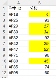
单元格值
单元格值条件格式 将格式应用于包含满足给定条件的值的每个单元格。 这有助于快速发现重要的数据点。
以下示例将单元格值条件格式应用于区域。 任何小于 60 的值都将更改单元格的填充颜色,并且字体变为斜体。
function main(workbook: ExcelScript.Workbook) {
    // Get the range to format.
    const sheet = workbook.getWorksheet("CellValue");
    const ratingColumn = sheet.getRange("B2:B12");
    sheet.activate();

    // Add cell value conditional formatting.
    const cellValueConditionalFormatting =
        ratingColumn.addConditionalFormat(ExcelScript.ConditionalFormatType.cellValue).getCellValue();

    // Create the condition, in this case when the cell value is less than 60
    let rule: ExcelScript.ConditionalCellValueRule = {
        formula1: "60",
        operator: ExcelScript.ConditionalCellValueOperator.lessThan
    };
    cellValueConditionalFormatting.setRule(rule);

    // Set the format to apply when the condition is met.
    let format = cellValueConditionalFormatting.getFormat();
    format.getFill().setColor("yellow");
    format.getFont().setItalic(true);
}
色阶
色阶条件格式 跨范围应用颜色渐变。 具有区域最小值和最大值的单元格使用指定的颜色,其他单元格按比例缩放。 可选的中点颜色提供更多对比度。
以下示例将红色、白色和蓝色刻度应用于所选区域。

function main(workbook: ExcelScript.Workbook) {
    // Get the range to format.
    const sheet = workbook.getWorksheet("ColorScale");
    const dataRange = sheet.getRange("B2:M13");
    sheet.activate();

    // Create a new conditional formatting object by adding one to the range.
    const conditionalFormatting = dataRange.addConditionalFormat(ExcelScript.ConditionalFormatType.colorScale);

    // Set the colors for the three parts of the scale: minimum, midpoint, and maximum.
    conditionalFormatting.getColorScale().setCriteria({
        minimum: {
            color: "#5A8AC6", /* A pale blue. */
            type: ExcelScript.ConditionalFormatColorCriterionType.lowestValue
        },
        midpoint: {
            color: "#FCFCFF", /* Slightly off-white. */
            formula: '=50', type: ExcelScript.ConditionalFormatColorCriterionType.percentile
        },
        maximum: {
            color: "#F8696B", /* A pale red. */
            type: ExcelScript.ConditionalFormatColorCriterionType.highestValue
        }
    });
}
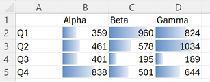
数据栏
数据条条件格式在 单元格的背景中添加部分填充的条形图。 条形图的填充度由单元格中的值和格式指定的区域定义。
以下示例在所选范围内创建数据栏条件格式。 数据条的比例从 0 到 1200。
function main(workbook: ExcelScript.Workbook) {
    // Get the range to format.
    const sheet = workbook.getWorksheet("DataBar");
    const dataRange = sheet.getRange("B2:D5");
    sheet.activate();

    // Create new conditional formatting on the range.
    const format = dataRange.addConditionalFormat(ExcelScript.ConditionalFormatType.dataBar);
    const dataBarFormat = format.getDataBar();

    // Set the lower bound of the data bar formatting to be 0.
    const lowerBound: ExcelScript.ConditionalDataBarRule = {
        type: ExcelScript.ConditionalFormatRuleType.number,
        formula: "0"
    };
    dataBarFormat.setLowerBoundRule(lowerBound);

    // Set the upper bound of the data bar formatting to be 1200.
    const upperBound: ExcelScript.ConditionalDataBarRule = {
        type: ExcelScript.ConditionalFormatRuleType.number,
        formula: "1200"
    };
    dataBarFormat.setUpperBoundRule(upperBound);
}
图标集
图标集条件格式 将图标添加到区域中的每个单元格。 图标来自指定的集。 图标基于有序的条件数组应用,每个条件映射到单个图标。
以下示例将设置条件格式的“三个交通灯”图标应用于范围。
![]()
function main(workbook: ExcelScript.Workbook) {
    // Get the range to format.
    const sheet = workbook.getWorksheet("IconSet");
    const dataRange = sheet.getRange("B2:B12");
    sheet.activate();

    // Create icon set conditional formatting on the range.
    const conditionalFormatting = dataRange.addConditionalFormat(ExcelScript.ConditionalFormatType.iconSet);

    // Use the "3 Traffic Lights (Unrimmed)" set.
    conditionalFormatting.getIconSet().setStyle(ExcelScript.IconSet.threeTrafficLights1);
    conditionalFormatting.getIconSet().setCriteria([
      { // Use the red light as the default for positive values.
        formula: '=0', operator: ExcelScript.ConditionalIconCriterionOperator.greaterThanOrEqual,
        type: ExcelScript.ConditionalFormatIconRuleType.number
      },
      { // The yellow light is applied to all values 6 and greater. The replaces the red light when applicable.
        formula: '=6', operator: ExcelScript.ConditionalIconCriterionOperator.greaterThanOrEqual,
        type: ExcelScript.ConditionalFormatIconRuleType.number
      },
      { // The green light is applied to all values 8 and greater. As with the yellow light, the icon is replaced when the new criteria is met.
        formula: '=8', operator: ExcelScript.ConditionalIconCriterionOperator.greaterThanOrEqual,
        type: ExcelScript.ConditionalFormatIconRuleType.number
      }
    ]);
}
预设
预设条件格式 根据常见方案(如空白单元格和重复值)将指定的格式应用于区域。 预设条件的完整列表由 ConditionalFormatPresetCriterion 枚举提供。
以下示例为区域中的任何空白单元格提供黄色填充。
function main(workbook: ExcelScript.Workbook) {
    // Get the range to format.
    const sheet = workbook.getWorksheet("Preset");
    const dataRange = sheet.getRange("B2:D5");
    sheet.activate();

    // Add new conditional formatting to that range.
    const conditionalFormat = dataRange.addConditionalFormat(
    ExcelScript.ConditionalFormatType.presetCriteria);

    // Set the conditional formatting to apply a yellow fill.
    const presetFormat = conditionalFormat.getPreset();
    presetFormat.getFormat().getFill().setColor("yellow");

    // Set a rule to apply the conditional format when cells are left blank.
    const blankRule: ExcelScript.ConditionalPresetCriteriaRule = {
        criterion: ExcelScript.ConditionalFormatPresetCriterion.blanks
    };
    presetFormat.setRule(blankRule);
}
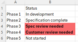
文本比较
文本比较条件格式 根据单元格的文本内容设置格式。 当文本以、包含、结尾或不包含给定子字符串时,将应用格式设置。
以下示例标记包含文本“review”的区域中的任何单元格。
function main(workbook: ExcelScript.Workbook) {
    // Get the range to format.
    const sheet = workbook.getWorksheet("TextComparison");
    const dataRange = sheet.getRange("B2:B6");
    sheet.activate();

    // Add conditional formatting based on the text in the cells.
    const textConditionFormat = dataRange.addConditionalFormat(
        ExcelScript.ConditionalFormatType.containsText).getTextComparison();

    // Set the conditional format to provide a light red fill and make the font bold.
    textConditionFormat.getFormat().getFill().setColor("#F8696B");
    textConditionFormat.getFormat().getFont().setBold(true);

    // Apply the condition rule that the text contains with "review".
    const textRule: ExcelScript.ConditionalTextComparisonRule = {
        operator: ExcelScript.ConditionalTextOperator.contains,
        text: "review"
    };
    textConditionFormat.setRule(textRule);
}
顶部/底部
上/下条件格式 标记区域中的最高值或最低值。 最高值和最低值基于原始值或百分比。
以下示例应用条件格式以显示区域中的两个最高数字。
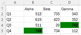
function main(workbook: ExcelScript.Workbook) {
  // Get the range to format.
  const sheet = workbook.getWorksheet("TopBottom");
  const dataRange = sheet.getRange("B2:D5");
  sheet.activate();

    // Set the fill color to green and the font to bold for the top 2 values in the range.
    const topBottomFormat = dataRange.addConditionalFormat(ExcelScript.ConditionalFormatType.topBottom).getTopBottom();
    topBottomFormat.getFormat().getFill().setColor("green");
    topBottomFormat.getFormat().getFont().setBold(true);
    topBottomFormat.setRule({
      rank: 2, /* The numeric threshold. */
      type: ExcelScript.ConditionalTopBottomCriterionType.topItems /* The type of the top/bottom condition. */
    });
}
自定义条件
自定义条件格式 允许在应用格式设置时定义复杂公式。 如果其他选项不够,请使用此选项。
以下示例针对所选区域设置自定义条件格式。 如果值大于行上一列中的值,则对单元格应用浅绿色填充和粗体字体。
function main(workbook: ExcelScript.Workbook) {
    // Get the range to format.
    const sheet = workbook.getWorksheet("Custom");
    const dataRange = sheet.getRange("B2:H2");
    sheet.activate();

    // Apply a rule for positive change from the previous column.
    const positiveChange = dataRange.addConditionalFormat(ExcelScript.ConditionalFormatType.custom).getCustom();
    positiveChange.getFormat().getFill().setColor("lightgreen");
    positiveChange.getFormat().getFont().setBold(true);
    positiveChange.getRule().setFormula(
        `=${dataRange.getCell(0, 0).getAddress()}>${dataRange.getOffsetRange(0, -1).getCell(0, 0).getAddress()}`
    );
}