Importing data with Microsoft R Server
In this blog, we would play around a new package RevoScaleR which takes a different approach in handling the data. Though, it works directly with flat files, but, is primarily made for a special kind of file format: XDF which enhances processing of the datasets.
RevoScaleR package stores the dataset on disk (hard drive) and loads it only a chunk at a time (where each chunk is a certain number of rows) for processing (reading or writing). Once a chunk is processed, it then moves to the next chunk of the data. By default, the chunk size is set to 500K rows, but we can increase decrease this size according to the number of columns in the dataset.
To summarize, data in RevoScaleR is external (because it's stored on disk) and distributed (because it's processed chunk-wise). This means we are no longer bound by memory when dealing with data: Our data can be as large as the space we have on the hard-disk to store it. Since at every point in time we only load one chunk of the data as a memory object (an R list object to be specific), we never overexert the system's memory.
Hand's-on
Pre-requisites:
1. Microsoft R Client(free): RevoScaleR works only with MRS which is an enterprise version. Hence, for only developing purpose, a free and a scaled down version of MRS is available called as Microsoft R Client. Though RevoScaleR works fine with it but not in full capacity.
2. To see how we can use Microsoft R Client to process and analyze a large dataset, we will be using trip data of January month of NYC Taxi dataset. This is a CSV file of 1.6GB with 10906858*19 dim.
Code(Ia): library(RevoScaleR) data_loc <- 'D:/MRS' input_csv <- file.path(data_loc, 'yellow_tripdata_2016-01.csv') st <- Sys.time() nyc_sample <- read.csv(input_csv) Sys.time() - st
Output(Ia):
> st <- Sys.time()
+ nyc_sample <- read.csv(input_csv)
+ Sys.time() - st
Time difference of 3.474699 mins
Code(Ib): st <- Sys.time() summary(nyc_sample) Sys.time() - st
Output(Ib):
> st <- Sys.time()
+ summary(nyc_sample)
+ Sys.time() - st
Time difference of 13.25179 secs
Code(IIa): input_xdf <- file.path(data_loc, 'yellow_tripdata_2016.xdf') st <- Sys.time() rxImport(input_csv, input_xdf, overwrite = TRUE) Sys.time() - st
Output(IIa): 
.xdf: 251,574 KB
.csv 1,668,628 KB
Notice the difference in the size of the both the files. We can further compress the .csv by setting the argument 'xdfCompressionLevel' but compressing it further would take extra time but again processing the more compressed version will be faster. Once the original CSV is converted to XDF, the runtime of processing (reading from and sometimes writing to) the XDF is shorter than what it would have been if we had directly processed the CSV instead. So, to decide whether we choose XDF or CSV we need to understand the I/O trade-offs.
This last code read the whole CSV file in just 1.9 min (compared to approx. 3.4 min in Code(Ia)) in chunks of 500K and created its XDF file in the working directory.
Output(IIa):
> st <- Sys.time()
+ rxImport(input_csv, input_xdf, overwrite = TRUE)
+ Sys.time() - st
Time difference of 1.900401 min
Code(IIb): Summary of all 19 columns
nyc_xdf <- RxXdfData(input_xdf) st <- Sys.time() rxSummary(~., nyc_xdf) Sys.time() - st
Output(IIb):
> st <- Sys.time()
+ rxSummary(~., nyc_xdf)
+ Sys.time() - st
Time difference of 11.75617 secs
Conclusion: 
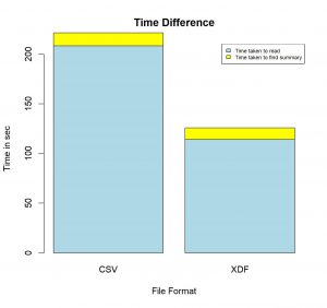
Blue Region : Time taken to read file
Yellow Region : Time taken to find summary
Finding summary of the 1.6GB CSV file took around 220 seconds, whereas, finding summary of the same file converted to the XDF format took only 125 seconds. This is when we tried finding only summary of the dataset. The time difference would vary by a very large factor when we would do some complex processing.
P.S: This is when we are using Microsoft R Client which has very limited capabilities. Processing speed of Microsoft R Server would touch great heights with multi-threaded and parallel processing.