Rapid Big Data Prototyping with Microsoft R Server on Apache Spark: Context Switching & Spark Tuning
Max Kaznady – Data Scientist; Jason Zhang – Senior Software Engineer;
Arijit Tarafdar – Senior Software Engineer; Miguel Fierro – Data Scientist
Introduction
During big data application development stage, it’s common to downsize the problem to the local machine for rapid code prototyping iterations. Developing machine learning models with Microsoft R Server (MRS) allows the user to quickly switch between code execution on the local machine and remote big data clusters such as Apache Spark on Azure HDInsight.
In this blog, we will demonstrate how to develop a predictive model for 170 million rows (37GB of raw data in Apache Hive) of the public NYC Taxi dataset fare data for 2013 using MRS’s local compute context, which will give us insight into which factors contribute to the taxi passenger tipping for the trip. We will show how easy it is to then train and execute the developed model at scale by switching the compute context to tuned Spark context – training at scale is on the order of 5 minutes with four Apache Spark D4_v2 series worker nodes (8 cores with 28GB of RAM each).
MRS compute context can also be switched to an SQL database and Hadoop Map Reduce - this blog's focus is MRS on Apache Spark.
Products
- HDInsight Apache Spark on Linux 1.6 cluster with Microsoft R Server installed on the edge node.
- RStudio GUI for R Server Studio, which is used to develop in Microsoft R Server on the edge node.
- MobaXterm client (or other SSH client such as Putty) to manage your SSH to MRS cluster.
Setup
First, you would have to spin up an MRS on Spark HDInsight cluster from Azure's portal – you can use the official guide to get started, or if you’re familiar with HDInsight clusters, you can just choose the options in Figure 1.
[caption id="attachment_2425" align="alignnone" width="582"] Figure 1: HDInsight Spark cluster configuration for Microsoft R Server.[/caption]
Once the cluster is created, you can connect to the edge node where MRS is already pre-installed by SSHing to r-server.YOURCLUSTERNAME-ssh.azurehdinsight.net with the credentials which you supplied during the cluster creation process. In order to do this in MobaXterm, you can go to Sessions, then New Sessions and then SSH.
The default installation of HDI Spark on Linux cluster does not come with RStudio Server installed on the edge node. RStudio Server is a popular open source integrated development environment (IDE) available for R that provides a browser-based IDE for use by remote clients. This tool allows you to benefit from all the power of R, Spark and Microsoft HDInsight cluster through your browser. In order to install RStudio you can follow the steps detailed in the guide, which reduces to running a script on the edge node.
After installing RStudio Server, all that remains to do is to setup an SSH tunnel to the edge node (we will use local port 8787 in this blog), which you will use to access RStudio Server locally on your machine. In order to create the tunnel with MobaXterm you have to press Tunneling and then “New SSH tunnel” - you will have to fill in the fields like in Figure 2.
[caption id="attachment_2445" align="alignnone" width="916"]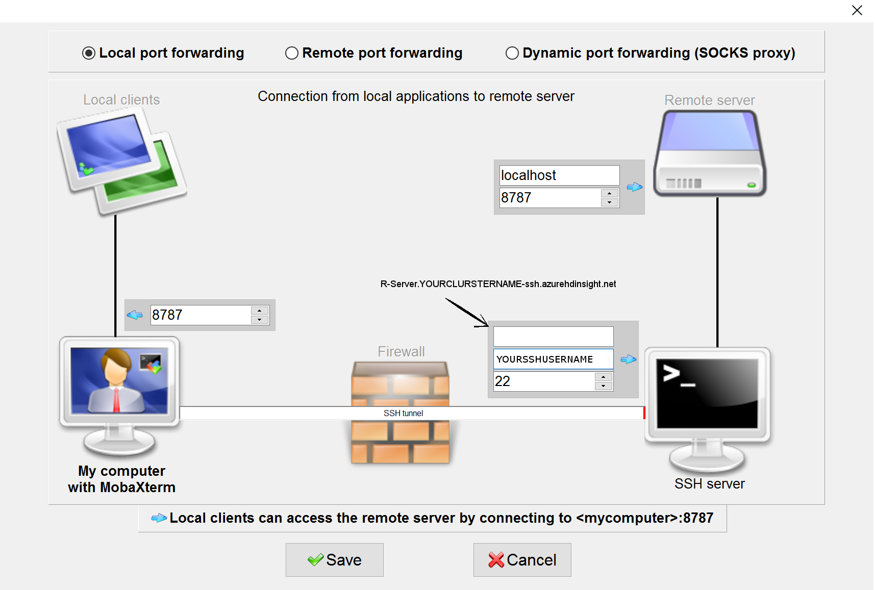 Figure 2: SSH tunnel configuration to access remotely RStudio in the HDInsight cluster.[/caption]
Alternatively you can create an SSH tunnel using Putty or, if you are using Linux (or Cygwin), you have to enter the following in your terminal:
ssh -f YOURSSHUSERNAME@r-server.YOURCLUSTERNAME-ssh.azurehdinsight.net -L 8787:localhost:8787 –N
Now you should be able to point a browser of your choice to localhost:8787 and login to the RStudio Server with your default edge node SSH credentials (The RStudio GUI should be already linked to Revo64 binary).
Data Preparation
We now have to prepare the raw NYC Taxi dataset for analysis. Largely, these steps have been outlined in the following post:
https://azure.microsoft.com/en-us/documentation/articles/machine-learning-data-science-process-hive-walkthrough
Also, there is a similar walkthrough for HDInsight Hadoop cluster which describes the use of Microsoft R Server with Hadoop compute context:
https://blog.revolutionanalytics.com/2016/04/mrs-nyc-taxi.html?no_prefetch=1
In this blog post, we specifically focus on Microsoft R Server solution using Apache Spark and context switching.
After you download and decompress the NYC Taxi trips and fares onto the edge node, you can use sample code to create the new Hive tables and to then load the data into them. After the data has been loaded, we need to join the trip and fare data.
Hive settings
The only non-default settings which we utilized for Hive was to switch the backend engine to Map Reduce
set hive.execution.engine=mr;
and view the headers on CLI (purely a convenience feature):
set hive.cli.print.header=true;
You can also place these settings into your .hiverc on the edge node.
Disclaimer
Normally, using Spark’s hiveContext we can stop here and simply query the underlying table to obtain train and test datasets. In the current release of MRS 8.0, this functionality is not yet supported, so we have to dump the Hive table data to WASB and then import it into MRS using rxImport function (thus re-imposing the schema); local context will work with one of Hive’s output files.
You can dump the joined table to WASB using these commands (obviously by substituting your storage account name and container into the script):
Context Preparation
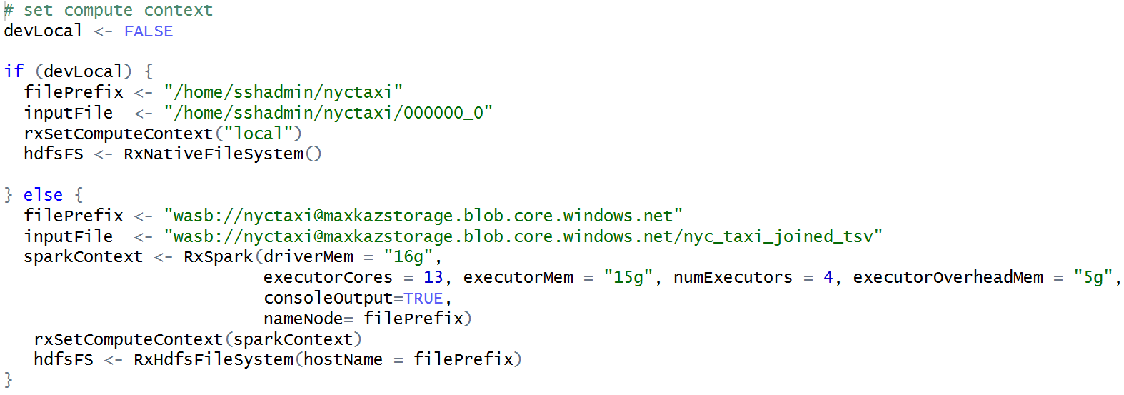
At this stage, the data has been loaded and we need to quickly iterate the models, so we add the following code for context switching:
We are now quickly able to develop the rest of the code around data manipulation and model building when devLocal is set to true; later we can switch the code to make it run at full scale by toggling devLocal to false.
Notice that we copied one of Hive table files for development purposes: nyctaxi/000000_0.
Data Manipulation
The data manipulation step was largely borrowed from the aforementioned tutorial of MRS on Hadoop, with a few exceptions.
First, we need to re-impose the data schema during the import stage, and drop variables which were used for feature engineering together with variables which are perfect predictors of whether or not the cab rider tipped.
Second, to make this interesting, we would also need to drop features which are near-perfect predictors of whether or not the cab passenger tipped. For example, Figure 2 shows that payment_type variable almost perfectly predicts the tip – cash payments almost never tip and credit card payments almost always tip. A more interesting problem to solve would be to figure out whether or not the person tips, independent of the payment type (the taxi driver has no control of what payment type the rider has).
[caption id="attachment_2305" align="alignnone" width="728"]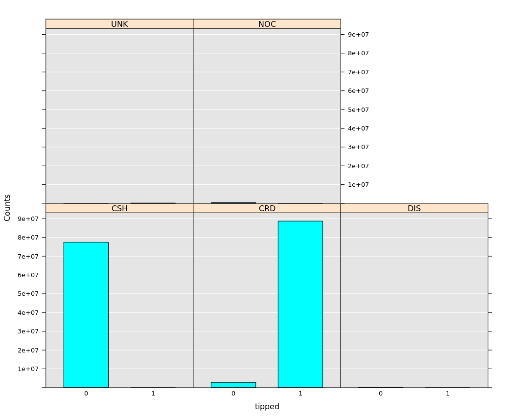 Figure 2: Histogram plot of payment_type and number of times the cab passenger tipped on reduced dataset using local MRS context.[/caption]
You can view the full source code which includes all these actions before proceeding further.
Machine Learning
Having defined our problem, we execute the decision tree algorithm and visualize the constructed tree, as well as feature importance. Please note that the decision tree plot is interactive and so we only showed the first few nodes in Figure 4.
Tree construction is consistent with the feature importance plot in Figure 3 – trip distance and hour of pickup seem to be influential predictors.
[caption id="attachment_2485" align="alignnone" width="658"]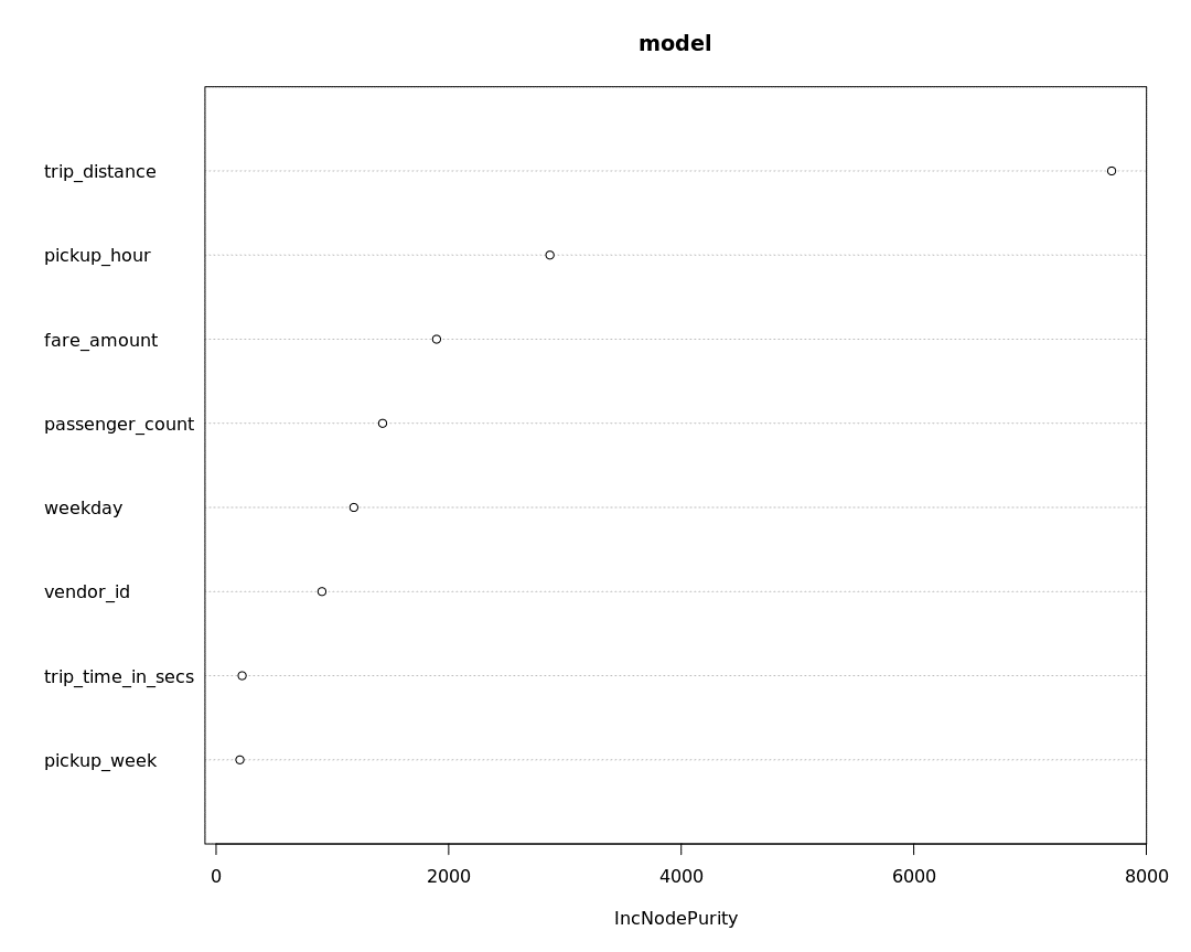 Figure 3: decision tree feature importance using local context on reduced dataset.[/caption]
[caption id="attachment_2495" align="alignnone" width="912"]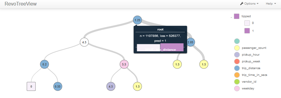 Figure 4: interactive decision tree visualization using local context on reduced dataset.[/caption]
Scaling to Spark
Recall that so far we were working with a local context and a reduced dataset – hence we were able to quickly hypothesize what the final solution should look like and what variables should be included. Now let’s see if our assumptions on a smaller dataset together with local compute context actually make sense on the full dataset.
However, scaling to Spark is not as simple as just toggling the devLocal switch – we need to know what Spark settings to set for RxSpark function and how they compare to usual Spark settings for MLlib.
Any Spark application will consume CPU cores and random access memory, hence tuning refers to controlling how resources are assigned to each executor running on each node. Our goals are:
- Achieve better parallelism on task execution.
- Cache data as much as possible in RDD.
- Minimize the impact of data rebuild.
- Avoid Out Of Memory (OOM) error on both on-heap and off-heap.
- Reduce network operation, e.g. shuffling.
There’s not a single solution for all scenarios, and the settings are based on many factors like cluster size, cluster node architecture, dataset size, algorithm, etc.
Since one has a fixed number of cores and memory for utilization, then using them all will maximize goals #1 and #2: cores maximize parallelism and memory size maximizes the size of the data which we cache off-disk.
For the remaining goals, we have two distinct Spark settings, with different pros and cons for each goal:
- Minimize the resource usage on each executor and create more executors:
With this approach, you can have minimal impact on rebuilding the data if the executor is lost, but you will have more data shuffling between executors and nodes, and potentially more OOM errors. - Maximize the resource usage on each executor and create fewer executors:
This will improve performance of goals #4 and #5, but degrade the performance during possible data recovery, as the executor is large and processes more data – hence if we lose such executor, we’ll need to perform a large amount of recovery work.
When Spark creates an executor container, the memory requested by each executor container is a total of spark.executor.memory (on-heap) + spark.yarn.executor.memoryOverhead (off-heap). Spark executor uses on-heap memory for execution, shuffle & storage and MRS is using off-heap memory to run MRS C++ code out of process – the results later get written to JVM filesystem.
For the RxSpark function (used to instantiate the connection to the Spark cluster), the default executor memory configuration is 4g/4g, meaning 4g of on-heap and 4g of off-heap memory. So you will see a total of 8g of memory allocated for each executor. The general guideline is a 1:1 mapping, but it is not always useful. It’s really hard to provide a precise ratio between the two, because the usage of off-heap memory depends on many factors like, the size of the dataset, algorithm, etc.
Advanced Caveats
If we have E executors (spark.executor.instances) and each of them has C cores (spark.executor.cores) and each task uses T CPUs (spark.task.cpus), then the amount of parallel execution slots is E x C / T.
Usually we don’t adjust T (default value is 1), and so usually the number of tasks which can run in parallel is E x C: hence there are two ways which can maximize this number
- Increase E
To do this, we need to decrease the memory usage of both on-heap and off-heap memory per executor. The maximum number of executors will be the lesser of
a) (total cores available) / (cores per executor)
b) (total memory available) / (on-heap + off-heap memory per executor) - Increase C
Start 1 executor per node, and use all available cores (for example, for D4_v2 series VMs used as worker nodes, YARN will allow 15 max cores per node, but you should choose 13 cores per executor - HDI cluster is already running other applications which are using some cores).
Clearly both approaches should consider the worker node boundaries, as one cannot merge the cores and memory of two different nodes to create an executor.
Other items need to be taken into consideration:
- With more tasks running in parallel on HDInsight cluster, storage account throttling may become an issue which may slow down the overall performance. For example, ingressing the data from disk (HDFS in our case) may throttle CPU utilization (the ultimate solution is Azure Data Lake, but one could also alleviate this bottleneck my manually stripping the data across multiple storage accounts).
- For MRS, the 1:1 ratio of on-heap / off-heap MRS memory usage is recommended, however not always. One can reduce the off-heap memory to achieve more executors or increase on-heap memory (for in-memory caching) as needed.
Spark Context
We’ve already adjusted the RxSpark and Spark settings for this problem, algorithm and default MRS on Spark hardware configuration (using four D4_v2 series worker nodes). The reader should refer to the previous section if they want to either work on a different problem, use a different algorithm or choose a different cluster configuration.
We switch the localDev to False and re-run our prototyped solution – the storage layer switches to WASB and the global compute context executes the rx functions against the Spark cluster. Final results in Figure 5, Figure 6 & Figure 7 are consistent with our earlier hypothesis.
Full source code is available from https://github.com/Azure/blog-mrs-spark-samples/blob/master/nyc_taxi_context_switch.R
We also developed a pySpark nodebook which benchmarks our results on MLlib on Spark. To be fair, we did not cache the dataframe in memory for a fair comparison of MLlib and MRS: caching takes about 4.5 minutes, but then MLlib training runtime cuts down to 3.7 minutes – overall the time is still slightly greater than rxDTree in Table 8, but comparable. The following is a link to full notebook, along with Spark settings:
https://github.com/Azure/blog-mrs-spark-samples/blob/master/MRS_MLlib_bench.ipynb
[caption id="attachment_2505" align="alignnone" width="755"] Figure 5: histogram by tip indicator for payment_type, performed on full dataset on Spark.[/caption]
[caption id="attachment_2506" align="alignnone" width="745"]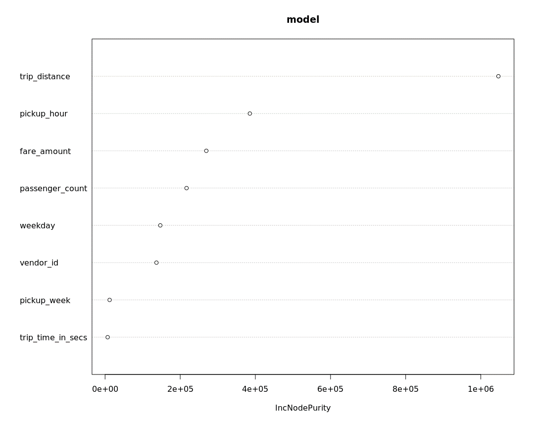 Figure 6: Feature importance with Spark context, formed by rxDTree model.[/caption]
[caption id="attachment_2516" align="alignnone" width="1309"]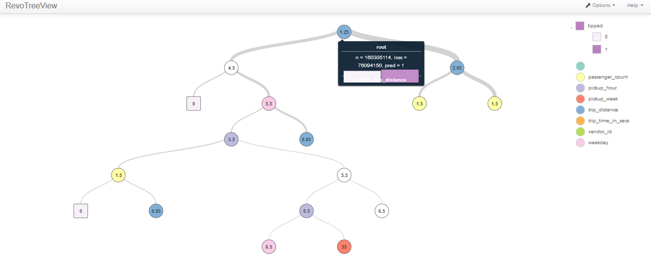 Figure 7: rxDTRee model partial plot, fitted on Spark to the training dataset.[/caption]
As we can see, both MRS and Spark provide comparable runtimes and F1 scores:
We can also plot the histograms of the two major predictors using Spark context, split by tip outcome (Figure 8). We see that trip distances of roughly 1 mile result in slightly higher likelihood of a tip being given, as probably most trips are of a distance of one mile – trip distributions by each tip indicator in Figure 8 are quite similar. We can hypothesize that this is probably because these trips occur in the downtown core, where passengers are more likely to tip anyway, but we’d need to analyze pickup and dropoff locations for that.
We also see in Figure 9 that passengers which are picked up after 9pm are more prone to tipping.
[caption id="attachment_2335" align="alignnone" width="768"]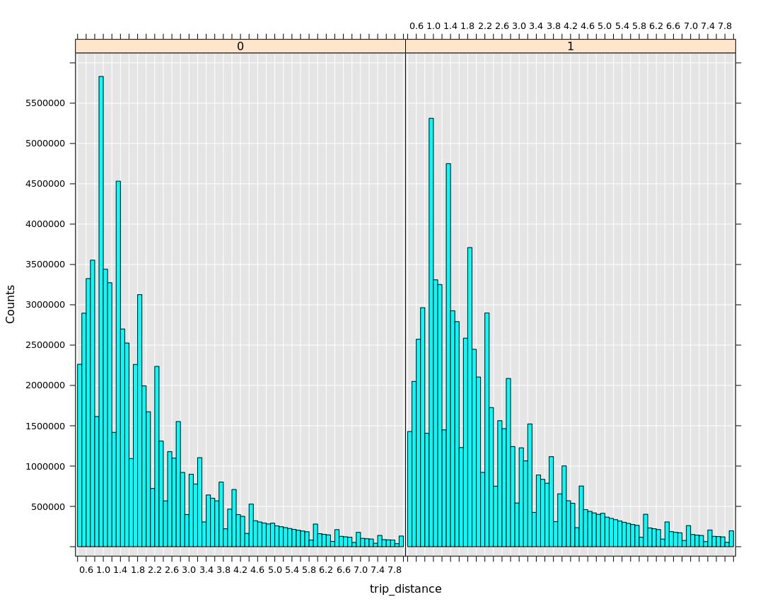 Figure 8: histograms trip distance split by tip indicator on full dataset.[/caption]
[caption id="attachment_2345" align="alignnone" width="770"] Figure 9: likelihood of a tip by pickup hour on the full data set.[/caption]
Conclusion
We were able to quickly develop a solution using MRS’s local context and then switch the solution to execute at full big data scale on Spark. We were able to also achieve comparable results to Spark’s MLlib algorithms. We can clearly identify that trip_distance and pickup_hour are influential predictors of whether the passenger tips or not.

