Ćwiczenie — szacowanie zasobów pod kątem rzeczywistego problemu
W poprzedniej lekcji przedstawiono podstawowe pojęcia narzędzia do szacowania zasobów kwantowych platformy Azure oraz sposób ich używania.
W tej lekcji oszacowasz zasoby wymagane do liczenia 2048-bitowej liczby całkowitej przy użyciu algorytmu Shora. Algorytm faktorowania Shora jest jednym z najbardziej znanych algorytmów kwantowych. Oferuje szybkość wykładniczą w przypadku dowolnego znanego klasycznego algorytmu faktorowania.
Klasyczna kryptografia używa środków fizycznych lub matematycznych, takich jak trudności obliczeniowe, do wykonania zadania. Popularnym protokołem kryptograficznym jest schemat Rivest-Shamir-Adleman (RSA), który opiera się na założeniu trudności z faktorowaniem liczb pierwszych przy użyciu komputera klasycznego.
Algorytm Shora sugeruje, że wystarczająco duże komputery kwantowe mogą przerwać kryptografię klucza publicznego. Szacowanie zasobów wymaganych przez algorytm Shora jest ważne, aby ocenić lukę w zabezpieczeniach tych typów schematów kryptograficznych.
W poniższym ćwiczeniu obliczysz szacowane zasoby dla współczynnika 2048-bitowej liczby całkowitej. W przypadku tej aplikacji obliczysz oszacowania zasobów fizycznych bezpośrednio z wstępnie skompilowanych oszacowań zasobów logicznych. W przypadku budżetu błędu użyjesz $\epsilon = 1/3$.
Pisanie algorytmuHora
W programie Visual Studio Code wybierz pozycję > poleceń i wybierz pozycję Utwórz: nowy notes Jupyter.
Zapisz notes jako ShorRE.ipynb.
W pierwszej komórce zaimportuj
qsharppakiet:import qsharpDodaj nową komórkę i skopiuj i wklej następujący kod:
%%qsharp
open Microsoft.Quantum.Arrays;
open Microsoft.Quantum.Canon;
open Microsoft.Quantum.Convert;
open Microsoft.Quantum.Diagnostics;
open Microsoft.Quantum.Intrinsic;
open Microsoft.Quantum.Math;
open Microsoft.Quantum.Measurement;
open Microsoft.Quantum.Unstable.Arithmetic;
open Microsoft.Quantum.ResourceEstimation;

operation RunProgram() : Unit {
    let bitsize = 31;

    // When choosing parameters for `EstimateFrequency`, make sure that
    // generator and modules are not co-prime
    let _ = EstimateFrequency(11, 2^bitsize - 1, bitsize);
}


// In this sample we concentrate on costing the `EstimateFrequency`
// operation, which is the core quantum operation in Shors algorithm, and
// we omit the classical pre- and post-processing.

/// # Summary
/// Estimates the frequency of a generator
/// in the residue ring Z mod `modulus`.
///
/// # Input
/// ## generator
/// The unsigned integer multiplicative order (period)
/// of which is being estimated. Must be co-prime to `modulus`.
/// ## modulus
/// The modulus which defines the residue ring Z mod `modulus`
/// in which the multiplicative order of `generator` is being estimated.
/// ## bitsize
/// Number of bits needed to represent the modulus.
///
/// # Output
/// The numerator k of dyadic fraction k/2^bitsPrecision
/// approximating s/r.
operation EstimateFrequency(
    generator : Int,
    modulus : Int,
    bitsize : Int
)
: Int {
    mutable frequencyEstimate = 0;
    let bitsPrecision =  2 * bitsize + 1;

    // Allocate qubits for the superposition of eigenstates of
    // the oracle that is used in period finding.
    use eigenstateRegister = Qubit[bitsize];

    // Initialize eigenstateRegister to 1, which is a superposition of
    // the eigenstates we are estimating the phases of.
    // We first interpret the register as encoding an unsigned integer
    // in little endian encoding.
    ApplyXorInPlace(1, eigenstateRegister);
    let oracle = ApplyOrderFindingOracle(generator, modulus, _, _);

    // Use phase estimation with a semiclassical Fourier transform to
    // estimate the frequency.
    use c = Qubit();
    for idx in bitsPrecision - 1..-1..0 {
        within {
            H(c);
        } apply {
            // `BeginEstimateCaching` and `EndEstimateCaching` are the operations
            // exposed by Azure Quantum Resource Estimator. These will instruct
            // resource counting such that the if-block will be executed
            // only once, its resources will be cached, and appended in
            // every other iteration.
            if BeginEstimateCaching("ControlledOracle", SingleVariant()) {
                Controlled oracle([c], (1 <<< idx, eigenstateRegister));
                EndEstimateCaching();
            }
            R1Frac(frequencyEstimate, bitsPrecision - 1 - idx, c);
        }
        if MResetZ(c) == One {
            set frequencyEstimate += 1 <<< (bitsPrecision - 1 - idx);
        }
    }

    // Return all the qubits used for oracles eigenstate back to 0 state
    // using Microsoft.Quantum.Intrinsic.ResetAll.
    ResetAll(eigenstateRegister);

    return frequencyEstimate;
}

/// # Summary
/// Interprets `target` as encoding unsigned little-endian integer k
/// and performs transformation |k⟩ ↦ |gᵖ⋅k mod N ⟩ where
/// p is `power`, g is `generator` and N is `modulus`.
///
/// # Input
/// ## generator
/// The unsigned integer multiplicative order ( period )
/// of which is being estimated. Must be co-prime to `modulus`.
/// ## modulus
/// The modulus which defines the residue ring Z mod `modulus`
/// in which the multiplicative order of `generator` is being estimated.
/// ## power
/// Power of `generator` by which `target` is multiplied.
/// ## target
/// Register interpreted as LittleEndian which is multiplied by
/// given power of the generator. The multiplication is performed modulo
/// `modulus`.
internal operation ApplyOrderFindingOracle(
    generator : Int, modulus : Int, power : Int, target : Qubit[]
)
: Unit
is Adj + Ctl {
    // The oracle we use for order finding implements |x⟩ ↦ |x⋅a mod N⟩. We
    // also use `ExpModI` to compute a by which x must be multiplied. Also
    // note that we interpret target as unsigned integer in little-endian
    // encoding by using the `LittleEndian` type.
    ModularMultiplyByConstant(modulus,
                                ExpModI(generator, power, modulus),
                                target);
}

/// # Summary
/// Performs modular in-place multiplication by a classical constant.
///
/// # Description
/// Given the classical constants `c` and `modulus`, and an input
/// quantum register (as LittleEndian) |𝑦⟩, this operation
/// computes `(c*x) % modulus` into |𝑦⟩.
///
/// # Input
/// ## modulus
/// Modulus to use for modular multiplication
/// ## c
/// Constant by which to multiply |𝑦⟩
/// ## y
/// Quantum register of target
internal operation ModularMultiplyByConstant(modulus : Int, c : Int, y : Qubit[])
: Unit is Adj + Ctl {
    use qs = Qubit[Length(y)];
    for (idx, yq) in Enumerated(y) {
        let shiftedC = (c <<< idx) % modulus;
        Controlled ModularAddConstant([yq], (modulus, shiftedC, qs));
    }
    ApplyToEachCA(SWAP, Zipped(y, qs));
    let invC = InverseModI(c, modulus);
    for (idx, yq) in Enumerated(y) {
        let shiftedC = (invC <<< idx) % modulus;
        Controlled ModularAddConstant([yq], (modulus, modulus - shiftedC, qs));
    }
}

/// # Summary
/// Performs modular in-place addition of a classical constant into a
/// quantum register.
///
/// # Description
/// Given the classical constants `c` and `modulus`, and an input
/// quantum register (as LittleEndian) |𝑦⟩, this operation
/// computes `(x+c) % modulus` into |𝑦⟩.
///
/// # Input
/// ## modulus
/// Modulus to use for modular addition
/// ## c
/// Constant to add to |𝑦⟩
/// ## y
/// Quantum register of target
internal operation ModularAddConstant(modulus : Int, c : Int, y : Qubit[])
: Unit is Adj + Ctl {
    body (...) {
        Controlled ModularAddConstant([], (modulus, c, y));
    }
    controlled (ctrls, ...) {
        // We apply a custom strategy to control this operation instead of
        // letting the compiler create the controlled variant for us in which
        // the `Controlled` functor would be distributed over each operation
        // in the body.
        //
        // Here we can use some scratch memory to save ensure that at most one
        // control qubit is used for costly operations such as `AddConstant`
        // and `CompareGreaterThenOrEqualConstant`.
        if Length(ctrls) >= 2 {
            use control = Qubit();
            within {
                Controlled X(ctrls, control);
            } apply {
                Controlled ModularAddConstant([control], (modulus, c, y));
            }
        } else {
            use carry = Qubit();
            Controlled AddConstant(ctrls, (c, y + [carry]));
            Controlled Adjoint AddConstant(ctrls, (modulus, y + [carry]));
            Controlled AddConstant([carry], (modulus, y));
            Controlled CompareGreaterThanOrEqualConstant(ctrls, (c, y, carry));
        }
    }
}

/// # Summary
/// Performs in-place addition of a constant into a quantum register.
///
/// # Description
/// Given a non-empty quantum register |𝑦⟩ of length 𝑛+1 and a positive
/// constant 𝑐 < 2ⁿ, computes |𝑦 + c⟩ into |𝑦⟩.
///
/// # Input
/// ## c
/// Constant number to add to |𝑦⟩.
/// ## y
/// Quantum register of second summand and target; must not be empty.
internal operation AddConstant(c : Int, y : Qubit[]) : Unit is Adj + Ctl {
    // We are using this version instead of the library version that is based
    // on Fourier angles to show an advantage of sparse simulation in this sample.

    let n = Length(y);
    Fact(n > 0, "Bit width must be at least 1");

    Fact(c >= 0, "constant must not be negative");
    Fact(c < 2 ^ n, $"constant must be smaller than {2L ^ n}");

    if c != 0 {
        // If c has j trailing zeroes than the j least significant bits
        // of y will not be affected by the addition and can therefore be
        // ignored by applying the addition only to the other qubits and
        // shifting c accordingly.
        let j = NTrailingZeroes(c);
        use x = Qubit[n - j];
        within {
            ApplyXorInPlace(c >>> j, x);
        } apply {
            IncByLE(x, y[j...]);
        }
    }
}

/// # Summary
/// Performs greater-than-or-equals comparison to a constant.
///
/// # Description
/// Toggles output qubit `target` if and only if input register `x`
/// is greater than or equal to `c`.
///
/// # Input
/// ## c
/// Constant value for comparison.
/// ## x
/// Quantum register to compare against.
/// ## target
/// Target qubit for comparison result.
///
/// # Reference
/// This construction is described in [Lemma 3, arXiv:2201.10200]
internal operation CompareGreaterThanOrEqualConstant(c : Int, x : Qubit[], target : Qubit)
: Unit is Adj+Ctl {
    let bitWidth = Length(x);

    if c == 0 {
        X(target);
    } elif c >= 2 ^ bitWidth {
        // do nothing
    } elif c == 2 ^ (bitWidth - 1) {
        ApplyLowTCNOT(Tail(x), target);
    } else {
        // normalize constant
        let l = NTrailingZeroes(c);

        let cNormalized = c >>> l;
        let xNormalized = x[l...];
        let bitWidthNormalized = Length(xNormalized);
        let gates = Rest(IntAsBoolArray(cNormalized, bitWidthNormalized));

        use qs = Qubit[bitWidthNormalized - 1];
        let cs1 = [Head(xNormalized)] + Most(qs);
        let cs2 = Rest(xNormalized);

        within {
            for i in IndexRange(gates) {
                (gates[i] ? ApplyAnd | ApplyOr)(cs1[i], cs2[i], qs[i]);
            }
        } apply {
            ApplyLowTCNOT(Tail(qs), target);
        }
    }
}

/// # Summary
/// Internal operation used in the implementation of GreaterThanOrEqualConstant.
internal operation ApplyOr(control1 : Qubit, control2 : Qubit, target : Qubit) : Unit is Adj {
    within {
        ApplyToEachA(X, [control1, control2]);
    } apply {
        ApplyAnd(control1, control2, target);
        X(target);
    }
}

internal operation ApplyAnd(control1 : Qubit, control2 : Qubit, target : Qubit)
: Unit is Adj {
    body (...) {
        CCNOT(control1, control2, target);
    }
    adjoint (...) {
        H(target);
        if (M(target) == One) {
            X(target);
            CZ(control1, control2);
        }
    }
}


/// # Summary
/// Returns the number of trailing zeroes of a number
///
/// ## Example
/// ```qsharp
/// let zeroes = NTrailingZeroes(21); // = NTrailingZeroes(0b1101) = 0
/// let zeroes = NTrailingZeroes(20); // = NTrailingZeroes(0b1100) = 2
/// ```
internal function NTrailingZeroes(number : Int) : Int {
    mutable nZeroes = 0;
    mutable copy = number;
    while (copy % 2 == 0) {
        set nZeroes += 1;
        set copy /= 2;
    }
    return nZeroes;
}

/// # Summary
/// An implementation for `CNOT` that when controlled using a single control uses
/// a helper qubit and uses `ApplyAnd` to reduce the T-count to 4 instead of 7.
internal operation ApplyLowTCNOT(a : Qubit, b : Qubit) : Unit is Adj+Ctl {
    body (...) {
        CNOT(a, b);
    }

    adjoint self;

    controlled (ctls, ...) {
        // In this application this operation is used in a way that
        // it is controlled by at most one qubit.
        Fact(Length(ctls) <= 1, "At most one control line allowed");

        if IsEmpty(ctls) {
            CNOT(a, b);
        } else {
            use q = Qubit();
            within {
                ApplyAnd(Head(ctls), a, q);
            } apply {
                CNOT(q, b);
            }
        }
    }

    controlled adjoint self;
}
Szacowanie algorytmu Shora
Teraz szacuj zasoby fizyczne dla RunProgram operacji przy użyciu domyślnych założeń. Dodaj nową komórkę i skopiuj i wklej następujący kod:
result = qsharp.estimate("RunProgram()")
result
Funkcja qsharp.estimate tworzy obiekt wynikowy, którego można użyć do wyświetlenia tabeli z ogólną liczbą zasobów fizycznych. Szczegóły kosztów można sprawdzić, zwijając grupy, które zawierają więcej informacji.
Na przykład zwiń grupę Parametrów kubitu logicznego, aby zobaczyć, że odległość kodu wynosi 21, a liczba kubitów fizycznych wynosi 882.
| Parametr kubitu logicznego | Wartość |
|---|---|
| Schemat QEC | surface_code |
| Odległość kodu | 21 |
| Kubity fizyczne | 882 |
| Czas cyklu logicznego | 8 milisek |
| Szybkość błędów kubitu logicznego | 3.00E-13 |
| Wstępna przeprawa | 0.03 |
| Próg korekty błędu | 0,01 |
| Formuła czasu cyklu logicznego | (4 * twoQubitGateTime + 2 * oneQubitMeasurementTime) * codeDistance |
| Formuła kubitów fizycznych | 2 * codeDistance * codeDistance |
Napiwek
W przypadku bardziej kompaktowej wersji tabeli wyjściowej można użyć polecenia result.summary.
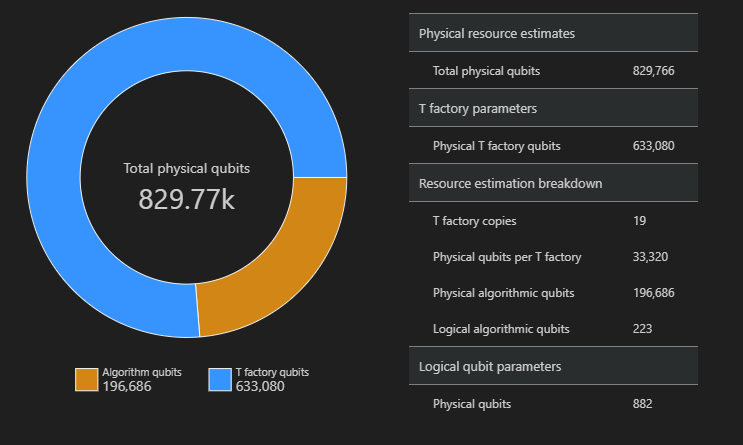
Wizualizowanie diagramu przestrzeni
Rozkład fizycznych kubitów używanych dla algorytmu i fabryk T jest czynnikiem, który może mieć wpływ na projekt algorytmu. Pakiet umożliwia qsharp-widgets wizualizowanie tej dystrybucji w celu lepszego zrozumienia szacowanych wymagań dotyczących przestrzeni algorytmu.
from qsharp_widgets import SpaceChart
SpaceChart(result)
W tym przykładzie liczba fizycznych kubitów wymaganych do uruchomienia algorytmu jest 829766, z których 196686 są kubitami algorytmów i 633080, z których są kubitami fabryki T.
Porównanie oszacowań zasobów dla różnych technologii kubitów
Narzędzie do szacowania zasobów usługi Azure Quantum umożliwia uruchamianie wielu konfiguracji parametrów docelowych i porównywanie wyników. Jest to przydatne, gdy chcesz porównać koszt różnych modeli kubitów, schematów QEC lub budżetów błędów.
Można również utworzyć listę parametrów szacowania przy użyciu EstimatorParams obiektu .
from qsharp.estimator import EstimatorParams, QubitParams, QECScheme, LogicalCounts

labels = ["Gate-based µs, 10⁻³", "Gate-based µs, 10⁻⁴", "Gate-based ns, 10⁻³", "Gate-based ns, 10⁻⁴", "Majorana ns, 10⁻⁴", "Majorana ns, 10⁻⁶"]

params = EstimatorParams(6)
params.error_budget = 0.333
params.items[0].qubit_params.name = QubitParams.GATE_US_E3
params.items[1].qubit_params.name = QubitParams.GATE_US_E4
params.items[2].qubit_params.name = QubitParams.GATE_NS_E3
params.items[3].qubit_params.name = QubitParams.GATE_NS_E4
params.items[4].qubit_params.name = QubitParams.MAJ_NS_E4
params.items[4].qec_scheme.name = QECScheme.FLOQUET_CODE
params.items[5].qubit_params.name = QubitParams.MAJ_NS_E6
params.items[5].qec_scheme.name = QECScheme.FLOQUET_CODE

qsharp.estimate("RunProgram()", params=params).summary_data_frame(labels=labels)
| Model kubitu | Kubity logiczne | Głębokość logiczna | Stany T | Odległość kodu | Fabryki T | Ułamek fabryki T | Kubity fizyczne | rQOPS | Środowisko uruchomieniowe fizyczne |
|---|---|---|---|---|---|---|---|---|---|
| Oparte na bramie μs, 10⁻³ | 223 3,64 mln | 4,70 mln | 17 | 13 | 40.54 % | 216,77 tys. | 21,86 tys. | 10 godzin | |
| Oparte na bramie μs, 10⁻⁴ | 223 | 3,64 mln | 4,70 mln | 9 | 14 | 43.17 % | 63,57 tys. | 41,30 tys. | 5 godzin |
| Ns oparte na bramie, 10⁻³ | 223 3,64 mln | 4,70 mln | 17 | 16 | 69.08 % | 416.89k | 32,79 mln | 25 s | |
| Ns oparte na bramie, 10⁻⁴ | 223 3,64 mln | 4,70 mln | 9 | 14 | 43.17 % | 63,57 tys. | 61,94 mln | 13 s | |
| Majorana ns, 10⁻⁴ | 223 3,64 mln | 4,70 mln | 9 | 19 | 82.75 % | 501.48k | 82,59 mln | 10 sekund | |
| Majorana ns, 10⁻⁶ | 223 3,64 mln | 4,70 mln | 5 | 13 | 31.47 % | 42,96 tys. | 148,67 mln | 5 s |
Wyodrębnianie oszacowań zasobów z liczby zasobów logicznych
Jeśli znasz już pewne oszacowania dla operacji, narzędzie do szacowania zasobów umożliwia uwzględnienie znanych oszacowań do ogólnego kosztu programu w celu skrócenia czasu wykonywania. Możesz użyć LogicalCounts klasy , aby wyodrębnić oszacowania zasobów logicznych z wstępnie obliczonych wartości szacowania zasobów.
Wybierz pozycję Kod , aby dodać nową komórkę, a następnie wprowadź i uruchom następujący kod:
logical_counts = LogicalCounts({
    'numQubits': 12581,
    'tCount': 12,
    'rotationCount': 12,
    'rotationDepth': 12,
    'cczCount': 3731607428,
    'measurementCount': 1078154040})

logical_counts.estimate(params).summary_data_frame(labels=labels)
| Model kubitu | Kubity logiczne | Głębokość logiczna | Stany T | Odległość kodu | Fabryki T | Ułamek fabryki T | Kubity fizyczne | Środowisko uruchomieniowe fizyczne |
|---|---|---|---|---|---|---|---|---|
| Oparte na bramie μs, 10⁻³ | 25481 | 1.2e+10 | 1.5e+10 | 27 | 13 | 0,6% | 37,38 mln | 6 lat |
| Oparte na bramie μs, 10⁻⁴ | 25481 | 1.2e+10 | 1.5e+10 | 13 | 14 | 0,8% | 8,68 mln | 3 lata |
| Ns oparte na bramie, 10⁻³ | 25481 | 1.2e+10 | 1.5e+10 | 27 | 15 | 1,3% | 37,65 mln | 2 dni |
| Ns oparte na bramie, 10⁻⁴ | 25481 | 1.2e+10 | 1.5e+10 | 13 | 18 | 1,2% | 8,72 mln | 18 godz. |
| Majorana ns, 10⁻⁴ | 25481 | 1.2e+10 | 1.5e+10 | 15 | 15 | 1,3% | 26,11 mln | 15 godzin |
| Majorana ns, 10⁻⁶ | 25481 | 1.2e+10 | 1.5e+10 | 7 | 13 | 0,5% | 6,25 mln | 7 godzin |
Podsumowanie
W najgorszym scenariuszu komputer kwantowy korzystający z kubitów opartych na bramie (kubitów, które mają czasy operacji w systemie nanosekund, takich jak nadkonduktowanie kubitów), a kod QEC powierzchni potrzebuje sześciu lat i 37,38 milionów kubitów, aby uwzględnić 2048-bitową liczbę całkowitą przy użyciu algorytmu Shora.
Jeśli używasz innej technologii kubitu — na przykład kubitów jonowych opartych na bramie — i tego samego kodu powierzchni, liczba kubitów nie zmienia się zbytnio, ale środowisko uruchomieniowe stanie się dwa dni w najgorszym przypadku i 18 godzin w optymistycznym przypadku. Jeśli zmienisz technologię kubitu i kod QEC — na przykład przy użyciu kubitów opartych na majoranie — współczynnik 2048-bitowej liczby całkowitej przy użyciu algorytmu Shora można wykonać w godzinach z tablicą 6,25 milionów kubitów w najlepszym przypadku scenariuszu.
Z eksperymentu możesz dowiedzieć się, że użycie kubitów Majorana i kodu QEC Floquet jest najlepszym wyborem do wykonania algorytmu I współczynnika 2048-bitowej liczby całkowitej.