Excelling in Excel: How to flip a column of data
I watch Twitter for interesting Microsoft Office productivity tips and problems, and I found one that's apparently a common issue: flipping a column of data in Excel.
If you simply want to reverse a list that's already in numeric or alphabetical order, that's easily done using Sort. And if you want to transpose columns to rows (or vice versa), just use the Transpose feature.
But what if you have a column of data that isn't sorted (and may even be in different formats: a mix of numbers and text) and you want to simply flip it so the bottommost items are on top and the top is now the bottom?
There are a number of ways to do this, including writing a macro, but the easiest way I can think of is to create a "helper column."
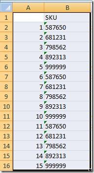
First, select the column you want to flip, right click it, and choose Insert to add your helper column. Now type "1" into the field next to the first piece of data you want to flip and "2" into the row below that. (If you have a header row and you want that to remain on top, start with the row just below it.) Now select both of those numbers and then double-click the lower right corner of the cell that contains the "2" to quickly fill down the length of your target column. (Or use the Fill, Series command on the Ribbon with a Linear Step Value of 1.)
Either way, you should end up with a numbered column, aka something you can sort that can be linked to your target column(s):

Select your helper column and any other columns you want sorted along with it. Go to the Data tab and click the Sort button and use this to Sort by your helper column using Largest to Smallest. That's it.
Once you're done, you could delete your helper column. But you might keep it to preserve a record of the original order of your data, in case you ever want to restore it (which can be useful if you perform lots of sorts on your data!). Right click it and select Hide if it gets in the way - you can always select the line between the columns and Unhide it if you ever need it back.
Suzanne
Comments
Anonymous
September 25, 2012
very helping tipAnonymous
November 21, 2012
Thank you!! Saved a lot of trouble!!Anonymous
January 04, 2013
thankyou! helped me so much and saved me the time and effort.Anonymous
February 07, 2013
very very helpful. you saved a lot of time, else I was thinking of typing 80 cells. :)Anonymous
February 23, 2013
Never mind, we found it! Thank you!Anonymous
March 17, 2013
does not work!Anonymous
May 11, 2013
This only sorted the helper column for me.Anonymous
May 26, 2013
its good my qustion is how to filp the cell it self lik durgham to show mahgrudAnonymous
June 18, 2013
smart trick for getting around one of the numerous essential missing features in Excel. ThanksAnonymous
July 03, 2013
Thanks! What a smart idea. It worked for me. That's what I did: select only the numbers on the help column (make sure your data correspond to the numbers in the help column) and then sort. Shall see a "Sort Warnning" dialogue window popping out. Then choose "Expand the section". By the way I did this on Excel 2010.Anonymous
September 20, 2013
Thank you! :)Anonymous
September 26, 2013
Doesn't want to work for Rows. Is there a similar solution for Rows?Anonymous
October 18, 2013
Thank you so much! I never thought this idea! Compared to OFFSET, your idea is really reliable! Thank u so much again, Suzanne!!!!Anonymous
October 31, 2013
For rows I would copy, paste by transposing, then do the trick of sorting, then copy by transposing again... never tested it but it should work! :-)Anonymous
November 20, 2013
Suzanne...You are the best....Danke Schöne!!