Excelling at Excel - Turning your data into a meaningful PivotChart
As we've seen in our examination on how to analyze your data, PivotTables are great when you want to dig into the numbers. But what if you want to present your data in a meaningful way for, say, an executive PowerPoint presentation.
You could make a regular chart. But if you don't know exactly the best way to present your data to make your point, you might spend a lot of time chart wrangling. A PivotChart can help you optimize your presentation much more efficiently.
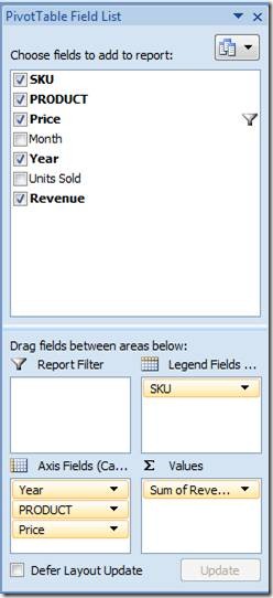
First, you don't need a PivotTable to create a PivotChart, though the way they work is very similar. Go to your data that's optimized for a PivotTable and select it (click the arrow at upper left to select all of the data on your active worksheet), click on the Insert tab, click the PivotTable button and select PivotChart from the dropdown list. Accept the defaults to create a new empty PivotChart worksheet with all your header row labels listed as fields:

Look familiar? Well, it's mostly the same as a PivotTable. Instead of Row Labels, you have Axis Fields (Categories). And there is Legend Field (Series) in place of Column Labels.
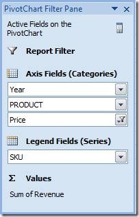
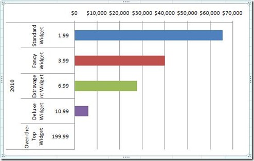
As with the PivotTable example, drag your key fields into Axis Fields (Categories). Order matters, but you can easily move things around until you get the result you want. I chose Year, Product, and then Price. The inclusion of this last field (which I didn't use in my PivotTable) neatly displays the price next to the sales totals, which helps communicate the impact of price on revenue:
To show the sales totals, I dragged Revenue down to Values. For some reason, Excel thought I wanted a Count of the data in this section so I clicked the down arrow, selected Value Field Settings, and converted it to a Sum. For Legend Fields, I entered SKU mainly to add a burst of color to the chart. If you want the actual legend displayed in your chart, go to the Layout tab and, in the Labels section, click the Legend button and then pick where you want it to appear.
You probably won't need Report Filter since PivotCharts are made to be filtered. When you click on your chart, you should see a box called PivotChart Filter Pane. If you don't see it (or if you ever close it or the Field List), simply go to the Analyze tab to toggle it back on.

From here, simply click the down arrow or filter icons next to the Axis Fields (Categories) to adjust what's displayed in your chart. You can add or subtract values and change the sort order.
If you want to manually re-order your axis items, first open the filter for the main category you want to adjust and click More Sort Options to select Manual. I needed to adjust the products so that they appear in price order with the Over-the-Tip Widget at the bottom.
Now here's the trick to make this work. When you created your PivotChart, you also made a companion PivotTable in the same worksheet. Select the cell in that table that contains the label for the section you want to shift (in my example, the Over-the-Top Widget). Now move your mouse to the upper right corner until you see the crosshair icon with arrows pointing up, down, left, and right. Now left-click and hold on the cell and then drag it up or down, using the gray line to identify its new prospective position. Find the spot where you want it to go and then release the mouse button to drop it there. Your chart will reflect the change you made to the table.
In most respects, PivotCharts are like regular Excel charts, so you can customize their appearance just as you would any chart for maximum impact in your presentation. But there are some advantages in how easily you can generate different views of your data to easily show, for example, annual and quarterly sales summaries.
Give it a try, and see just how quickly you can build different views from the same data to make your point.
Suzanne
