SharePoint 2010: How to Export SharePoint List to Excel Sheet as Records and Charts
Introduction
Microsoft office tools are most famous and widely used all over the world in offices. So it’s no surprise that Office tools can be used in or can use other Microsoft products. So is SharePoint. Excel application amongst the Office tool is most used by people in offices to store records, to create the charts, reports. So in this article we are going to see how we can get data into excel sheet from the SharePoint list.
Problem
So let’s say your manager comes and ask you that he wants single excel file in which there will be multiple sheets which will be linked to separate single SharePoint list and will fetch all records from there. And he/she wants it quickly and no need of new application. Now as a developer you will first think what Manager is saying? Without writing new application? Is there any way I can do this quickly? Yes you can do this by some tricks.
Solutions
Yes you can achieve this requirement with the help of SharePoint list and Excel. What you need is just follow below steps. Before starting let’s take two lists: A and B for our example. So the Problem statement will be like: fetch data of list A into Sheet1 and data of list B into Sheet2. Let’s start with below steps:
1. Go to SharePoint List A and then click on List tab on Ribbon control
2. Then click on ‘Export to Excel’ button on ribbon control
3. Save the file with meaningful name, for example: owssvrA.
4. Repeat the steps for 1 to 3 for List B and save file with another name: owssvrB.
5. Now we have 'MS Excel Web Query File' files for both lists.
6. Open new excel application.
7. Go to Sheet1 and click on any cell.
8. Click on Data in ribbon
9. Click on Existing Data Connection
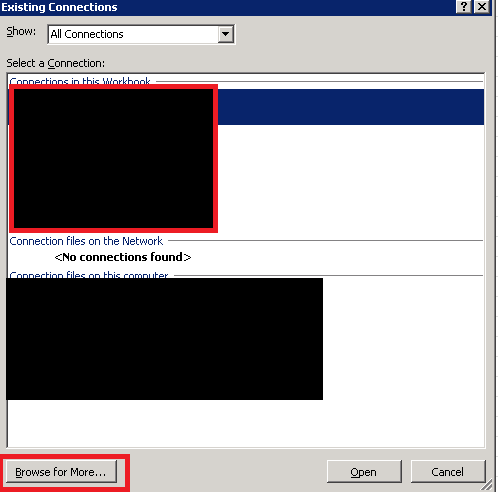
10. Click on ‘Browse for More’ and go to the location where ‘'MS Excel Web Query File’ files are saved.
11. Select List A’s Query File and click Open.
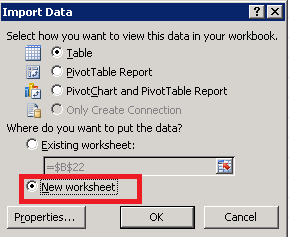
12. On Import Data pop up select ‘New Worksheet’, (if you know exact column numbers then choose existing worksheet and cell range).
13. Now you have data of List in your Excel sheet.
14. Rename sheet with name: “Sheet1” and you are done for list A.
15. Now repeat same steps for List B and you have two lists data in two separate sheets. You can refresh data as well from the ribbon button. Isn’t it easy?? And once this is done you have this for forever to use. This is best solution for those who are comfortable with the excel sheet. You can also create the chart with above approach; only there is slightly change after step 11. Let’s do it also, so steps onwards 12 will be like:
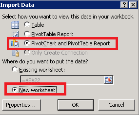
12. On Import Data pop up choose ‘Pivot Chart and Pivot table Report’ and ‘New worksheet’.
13. Then click on the OK button. And it will open new sheet with chart configuration wizard. Just configure how you want your chart and you are done. You can also refresh your charts/reports so that latest data from list can be taken. You have refresh button under Data tab on ribbon control. So without writing single line of code and minimal effort you have implemented great solution for your manager. Isn’t it great?


