チュートリアル: レコメンデーション システムを作成、評価、スコア付けする
このチュートリアルでは、Microsoft Fabric の Synapse Data Science ワークフローのエンド ツー エンドの例を示します。 このシナリオでは、オンラインブックのレコメンデーションのモデルを構築します。
このチュートリアルでは、次の手順について説明します。
- レイクハウスにデータをアップロードする
- データに対して探索的分析を実行する
- モデルをトレーニングし、MLflow でログに記録する
- モデルを読み込んで予測を行う
さまざまな種類の推奨アルゴリズムを使用できます。 このチュートリアルでは、交互最小二乗 (ALS) 行列分解アルゴリズムを使用します。 ALS は、モデルベースのコラボレーション フィルタリング アルゴリズムです。

ALS は、評価行列 R を、2 つの下位ランク行列である you と V の積として推定しようとします。ここでは、R = U * Vt です。 通常、これらの近似値は、因子 行列と呼ばれます。
ALS アルゴリズムは反復的です。 各反復は係数行列の一方の定数を保持し、他方は最小二乗法を使用して解決します。 次に、新しく解いた因子行列定数を保持し、他方の因子行列を解きます。

前提 条件
Microsoft Fabric サブスクリプションを取得します。 または、無料で Microsoft Fabric 試用版 にサインアップします。
Microsoft Fabric にサインインします。
ホーム ページの左下にあるエクスペリエンス スイッチャーを使用して、Fabric に切り替えます。
- 必要に応じて、Microsoft Fabric でレイクハウスを作成するには、「Microsoft Fabricのレイクハウス作成」に関する説明に従ってください。
ノートに書きながら進めてください。
次のいずれかのオプションを選択してノートブックで作業を進めます。
- 組み込みのノートブックを開いて実行します。
- GitHub からノートブックをアップロードします。
組み込みのノートブックを開く
「サンプル の読書推奨ノート は、このチュートリアルに付属しています。」
このチュートリアルのサンプルノートブックを開くには、「データサイエンス用にシステムを準備する」の手順に従ってください。
コードの実行を開始する前に、必ずレイクハウスをノートブックにアタッチしてください。
GitHub からノートブックをインポートする
このチュートリアルには、AIsample - Book Recommendation.ipynb ノートブックが付属しています。
このチュートリアルの付属のノートブックを開くには、「データ サイエンス用にシステムを準備する」の手順に従って、ノートブックをワークスペースにインポート します。
このページからコードをコピーして貼り付ける場合は、新しいノートブックを作成することができます。
コードの実行を開始する前に、必ずレイクハウスをノートブックにアタッチしてください。
手順 1: データを読み込む
このシナリオの書籍のレコメンデーション データセットは、次の 3 つの独立したデータセットで構成されています。
Books.csv: 国際標準書番号 (ISBN) は、無効な日付が既に削除されている各書籍を識別します。 データ セットには、タイトル、作成者、発行元も含まれます。 複数の著者が含まれる書籍の場合、Books.csv ファイルには最初の著者のみが一覧表示されます。 URL は、3 つのサイズのカバー画像の Amazon Web サイト リソースを指します。
ISBN Book-Title Book-Author Year-Of-Publication 発行者 Image-URL-S Image-URL-M Image-URL-l 0195153448 古典的神話 Mark P. O. Morford 2002 オックスフォード大学出版局 http://images.amazon.com/images/P/0195153448.01.THUMBZZZ.jpg http://images.amazon.com/images/P/0195153448.01.MZZZZZZZ.jpg http://images.amazon.com/images/P/0195153448.01.LZZZZZZZ.jpg 0002005018 クララ カラン リチャード・ブルース・ライト 2001 ハーパーフラミングオ カナダ http://images.amazon.com/images/P/0002005018.01.THUMBZZZ.jpg http://images.amazon.com/images/P/0002005018.01.MZZZZZZZ.jpg http://images.amazon.com/images/P/0002005018.01.LZZZZZZZ.jpg Ratings.csv: 各書籍の評価は、明示的 (ユーザーによって提供され、1 から 10 のスケールで提供) または暗黙的 (ユーザー入力なしで観察され、0 で示されます) のいずれかです。
User-ID ISBN Book-Rating 276725 034545104X 0 276726 0155061224 5 Users.csv: ユーザー ID は匿名化され、整数にマップされます。 人口統計データ (場所や年齢など) が提供されます (利用可能な場合)。 このデータが使用できない場合、これらの値は
null。User-ID 場所 年齢 1 "nyc new york usa" 2 "stockton california usa" 18.0
さまざまなデータセットでこのノートブックを使用できるように、これらのパラメーターを定義します。
IS_CUSTOM_DATA = False  # If True, the dataset has to be uploaded manually

USER_ID_COL = "User-ID"  # Must not be '_user_id' for this notebook to run successfully
ITEM_ID_COL = "ISBN"  # Must not be '_item_id' for this notebook to run successfully
ITEM_INFO_COL = (
    "Book-Title"  # Must not be '_item_info' for this notebook to run successfully
)
RATING_COL = (
    "Book-Rating"  # Must not be '_rating' for this notebook to run successfully
)
IS_SAMPLE = True  # If True, use only <SAMPLE_ROWS> rows of data for training; otherwise, use all data
SAMPLE_ROWS = 5000  # If IS_SAMPLE is True, use only this number of rows for training

DATA_FOLDER = "Files/book-recommendation/"  # Folder that contains the datasets
ITEMS_FILE = "Books.csv"  # File that contains the item information
USERS_FILE = "Users.csv"  # File that contains the user information
RATINGS_FILE = "Ratings.csv"  # File that contains the rating information

EXPERIMENT_NAME = "aisample-recommendation"  # MLflow experiment name
データをダウンロードしてレイクハウスに格納する
このコードはデータセットをダウンロードし、それを lakehouse に格納します。
重要
実行する前にノートブックにレイクハウスを追加してください。 それ以外の場合は、エラーが発生します。
if not IS_CUSTOM_DATA:
    # Download data files into a lakehouse if they don't exist
    import os, requests

    remote_url = "https://synapseaisolutionsa.blob.core.windows.net/public/Book-Recommendation-Dataset"
    file_list = ["Books.csv", "Ratings.csv", "Users.csv"]
    download_path = f"/lakehouse/default/{DATA_FOLDER}/raw"

    if not os.path.exists("/lakehouse/default"):
        raise FileNotFoundError(
            "Default lakehouse not found, please add a lakehouse and restart the session."
        )
    os.makedirs(download_path, exist_ok=True)
    for fname in file_list:
        if not os.path.exists(f"{download_path}/{fname}"):
            r = requests.get(f"{remote_url}/{fname}", timeout=30)
            with open(f"{download_path}/{fname}", "wb") as f:
                f.write(r.content)
    print("Downloaded demo data files into lakehouse.")
MLflow 実験の追跡を設定する
このコードを使用して、MLflow 実験の追跡を設定します。 この例では、自動ログ記録を無効にします。 詳細については、Microsoft Fabric の 自動ログ記録に関する記事を参照してください。
# Set up MLflow for experiment tracking
import mlflow

mlflow.set_experiment(EXPERIMENT_NAME)
mlflow.autolog(disable=True)  # Disable MLflow autologging
レイクハウスからデータを読み取る
適切なデータが lakehouse に配置されたら、3 つのデータセットをノートブック内の個別の Spark DataFrames に読み取ります。 このコードのファイル パスでは、前に定義したパラメーターを使用します。
df_items = (
    spark.read.option("header", True)
    .option("inferSchema", True)
    .csv(f"{DATA_FOLDER}/raw/{ITEMS_FILE}")
    .cache()
)

df_ratings = (
    spark.read.option("header", True)
    .option("inferSchema", True)
    .csv(f"{DATA_FOLDER}/raw/{RATINGS_FILE}")
    .cache()
)

df_users = (
    spark.read.option("header", True)
    .option("inferSchema", True)
    .csv(f"{DATA_FOLDER}/raw/{USERS_FILE}")
    .cache()
)
手順 2: 探索的データ分析を実行する
生データを表示する
display コマンドを使用して DataFrames を探索します。 このコマンドを使用すると、高レベルの DataFrame 統計を表示し、さまざまなデータセット列が相互にどのように関連しているかを理解できます。 データセットを調べる前に、次のコードを使用して必要なライブラリをインポートします。
import pyspark.sql.functions as F
from pyspark.ml.feature import StringIndexer
import matplotlib.pyplot as plt
import seaborn as sns
color = sns.color_palette()  # Adjusting plotting style
import pandas as pd  # DataFrames
このコードを使用して、書籍データを含む DataFrame を確認します。
display(df_items, summary=True)
後で使用するために、_item_id 列を追加します。 _item_id 値は、推奨モデルの整数である必要があります。 このコードでは、StringIndexer を使用して ITEM_ID_COL をインデックスに変換します。
df_items = (
    StringIndexer(inputCol=ITEM_ID_COL, outputCol="_item_id")
    .setHandleInvalid("skip")
    .fit(df_items)
    .transform(df_items)
    .withColumn("_item_id", F.col("_item_id").cast("int"))
)
DataFrame を表示し、_item_id 値が期待どおりに単調に連続して増加するかどうかを確認します。
display(df_items.sort(F.col("_item_id").desc()))
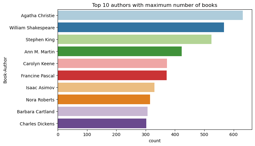
このコードを使用して、上位 10 人の著者を、書かれた書籍の数で降順にプロットします。 アガサ・クリスティは、600冊以上の本を持ち、その後ウィリアム・シェイクスピアが続く主要著者です。
df_books = df_items.toPandas() # Create a pandas DataFrame from the Spark DataFrame for visualization
plt.figure(figsize=(8,5))
sns.countplot(y="Book-Author",palette = 'Paired', data=df_books,order=df_books['Book-Author'].value_counts().index[0:10])
plt.title("Top 10 authors with maximum number of books")
次に、ユーザー データを含む DataFrame を表示します。
display(df_users, summary=True)
行に不足している User-ID 値がある場合は、その行を削除します。 カスタマイズされたデータセットに値がない場合でも、問題は発生しません。
df_users = df_users.dropna(subset=(USER_ID_COL))
display(df_users, summary=True)
後で使用するために、_user_id 列を追加します。 推奨モデルの場合、_user_id 値は整数である必要があります。 次のコード サンプルでは、StringIndexer を使用して USER_ID_COL をインデックスに変換します。
ブックデータセットには、既に整数の列 User-ID が含まれています。 ただし、異なるデータセットとの互換性のために _user_id 列を追加すると、この例はより堅牢になります。 次のコードを使用して、_user_id 列を追加します。
df_users = (
    StringIndexer(inputCol=USER_ID_COL, outputCol="_user_id")
    .setHandleInvalid("skip")
    .fit(df_users)
    .transform(df_users)
    .withColumn("_user_id", F.col("_user_id").cast("int"))
)
display(df_users.sort(F.col("_user_id").desc()))
評価データを表示するには、次のコードを使用します。
display(df_ratings, summary=True)
個別の評価を取得し、後で使用するために ratingsという名前のリストに保存します。
ratings = [i[0] for i in df_ratings.select(RATING_COL).distinct().collect()]
print(ratings)
次のコードを使用して、評価が最も高い上位 10 冊の書籍を表示します。
plt.figure(figsize=(8,5))
sns.countplot(y="Book-Title",palette = 'Paired',data= df_books, order=df_books['Book-Title'].value_counts().index[0:10])
plt.title("Top 10 books per number of ratings")
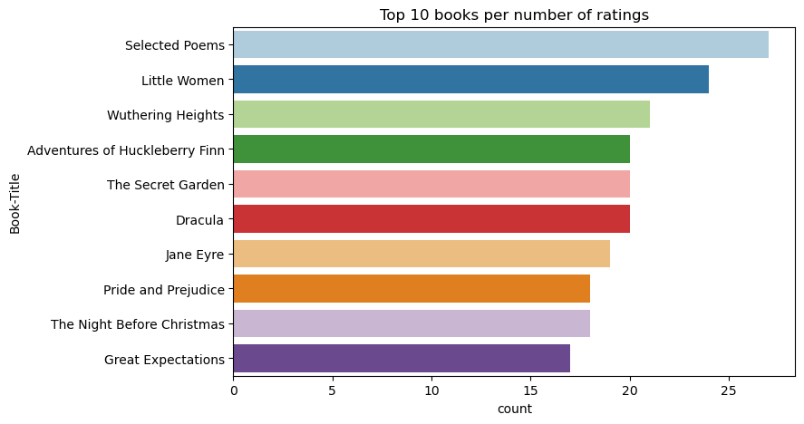
評価によると、選択された詩 は最も人気のある本です。 アドベンチャーズ オブ ハックルベリー フィン、シークレット ガーデン、ドラキュラ の評価は同じです。
データのマージ
より包括的な分析のために、3 つの DataFrame を 1 つの DataFrame にマージします。
df_all = df_ratings.join(df_users, USER_ID_COL, "inner").join(
    df_items, ITEM_ID_COL, "inner"
)
df_all_columns = [
    c for c in df_all.columns if c not in ["_user_id", "_item_id", RATING_COL]
]

# Reorder the columns to ensure that _user_id, _item_id, and Book-Rating are the first three columns
df_all = (
    df_all.select(["_user_id", "_item_id", RATING_COL] + df_all_columns)
    .withColumn("id", F.monotonically_increasing_id())
    .cache()
)

display(df_all)
このコードを使用して、個別のユーザー、書籍、操作の数を表示します。
print(f"Total Users: {df_users.select('_user_id').distinct().count()}")
print(f"Total Items: {df_items.select('_item_id').distinct().count()}")
print(f"Total User-Item Interactions: {df_all.count()}")
最も人気のある項目を計算してプロットする
このコードを使用して、最も人気のある書籍の上位 10 件を計算して表示します。
# Compute top popular products
df_top_items = (
    df_all.groupby(["_item_id"])
    .count()
    .join(df_items, "_item_id", "inner")
    .sort(["count"], ascending=[0])
)

# Find top <topn> popular items
topn = 10
pd_top_items = df_top_items.limit(topn).toPandas()
pd_top_items.head(10)
ヒント
<topn> の値を、[人気度] または [売れ筋] レコメンデーション セクションに使用します。
# Plot top <topn> items
f, ax = plt.subplots(figsize=(10, 5))
plt.xticks(rotation="vertical")
sns.barplot(y=ITEM_INFO_COL, x="count", data=pd_top_items)
ax.tick_params(axis='x', rotation=45)
plt.xlabel("Number of Ratings for the Item")
plt.show()

トレーニング データセットとテスト データセットを準備する
ALS マトリックスでは、トレーニング前にデータの準備が必要です。 このコード サンプルを使用して、データを準備します。 このコードでは、次のアクションを実行します。
- 評価列を正しい型にキャストする
- ユーザー評価を使用してトレーニング データをサンプリングする
- データをトレーニング データセットとテスト データセットに分割する
if IS_SAMPLE:
    # Must sort by '_user_id' before performing limit to ensure that ALS works normally
    # If training and test datasets have no common _user_id, ALS will fail
    df_all = df_all.sort("_user_id").limit(SAMPLE_ROWS)

# Cast the column into the correct type
df_all = df_all.withColumn(RATING_COL, F.col(RATING_COL).cast("float"))

# Using a fraction between 0 and 1 returns the approximate size of the dataset; for example, 0.8 means 80% of the dataset
# Rating = 0 means the user didn't rate the item, so it can't be used for training
# We use the 80% of the dataset with rating > 0 as the training dataset
fractions_train = {0: 0}
fractions_test = {0: 0}
for i in ratings:
    if i == 0:
        continue
    fractions_train[i] = 0.8
    fractions_test[i] = 1
# Training dataset
train = df_all.sampleBy(RATING_COL, fractions=fractions_train)

# Join with leftanti will select all rows from df_all with rating > 0 and not in the training dataset; for example, the remaining 20% of the dataset
# test dataset
test = df_all.join(train, on="id", how="leftanti").sampleBy(
    RATING_COL, fractions=fractions_test
)
スパリティとは、ユーザーの関心事の類似性を識別できない疎なフィードバック データを指します。 データと現在の問題の両方について理解を深めるために、次のコードを使用してデータセットのスパリティを計算します。
# Compute the sparsity of the dataset
def get_mat_sparsity(ratings):
    # Count the total number of ratings in the dataset - used as numerator
    count_nonzero = ratings.select(RATING_COL).count()
    print(f"Number of rows: {count_nonzero}")

    # Count the total number of distinct user_id and distinct product_id - used as denominator
    total_elements = (
        ratings.select("_user_id").distinct().count()
        * ratings.select("_item_id").distinct().count()
    )

    # Calculate the sparsity by dividing the numerator by the denominator
    sparsity = (1.0 - (count_nonzero * 1.0) / total_elements) * 100
    print("The ratings DataFrame is ", "%.4f" % sparsity + "% sparse.")

get_mat_sparsity(df_all)
# Check the ID range
# ALS supports only values in the integer range
print(f"max user_id: {df_all.agg({'_user_id': 'max'}).collect()[0][0]}")
print(f"max user_id: {df_all.agg({'_item_id': 'max'}).collect()[0][0]}")
手順 3: モデルを開発してトレーニングする
ALS モデルをトレーニングして、ユーザーにパーソナライズされた推奨事項を提供します。
モデルを定義する
Spark ML には、ALS モデルを構築するための便利な API が用意されています。 ただし、このモデルでは、データのスパリティやコールド スタートなどの問題を確実に処理しません (ユーザーまたは項目が新しい場合に推奨事項を作成します)。 モデルのパフォーマンスを向上させるには、クロス検証とハイパーパラメーターの自動チューニングを組み合わせます。
このコードを使用して、モデルのトレーニングと評価に必要なライブラリをインポートします。
# Import Spark required libraries
from pyspark.ml.evaluation import RegressionEvaluator
from pyspark.ml.recommendation import ALS
from pyspark.ml.tuning import ParamGridBuilder, CrossValidator, TrainValidationSplit

# Specify the training parameters
num_epochs = 1  # Number of epochs; here we use 1 to reduce the training time
rank_size_list = [64]  # The values of rank in ALS for tuning
reg_param_list = [0.01, 0.1]  # The values of regParam in ALS for tuning
model_tuning_method = "TrainValidationSplit"  # TrainValidationSplit or CrossValidator
# Build the recommendation model by using ALS on the training data
# We set the cold start strategy to 'drop' to ensure that we don't get NaN evaluation metrics
als = ALS(
    maxIter=num_epochs,
    userCol="_user_id",
    itemCol="_item_id",
    ratingCol=RATING_COL,
    coldStartStrategy="drop",
    implicitPrefs=False,
    nonnegative=True,
)
モデルハイパーパラメーターの調整
次のコード サンプルでは、ハイパーパラメーターの検索に役立つパラメーター グリッドを構築します。 また、このコードでは、評価メトリックとしてルート平均二乗誤差 (RMSE) を使用する回帰エバリュエーターも作成されます。
#  Construct a grid search to select the best values for the training parameters
param_grid = (
    ParamGridBuilder()
    .addGrid(als.rank, rank_size_list)
    .addGrid(als.regParam, reg_param_list)
    .build()
)

print("Number of models to be tested: ", len(param_grid))

# Define the evaluator and set the loss function to the RMSE
evaluator = RegressionEvaluator(
    metricName="rmse", labelCol=RATING_COL, predictionCol="prediction"
)
次のコード サンプルでは、構成済みのパラメーターに基づいて、さまざまなモデル チューニング 方法を開始します。 モデルのチューニングの詳細については、Apache Spark Web サイトの「ML チューニング: モデルの選択とハイパーパラメーターの調整」を参照してください。
# Build cross-validation by using CrossValidator and TrainValidationSplit
if model_tuning_method == "CrossValidator":
    tuner = CrossValidator(
        estimator=als,
        estimatorParamMaps=param_grid,
        evaluator=evaluator,
        numFolds=5,
        collectSubModels=True,
    )
elif model_tuning_method == "TrainValidationSplit":
    tuner = TrainValidationSplit(
        estimator=als,
        estimatorParamMaps=param_grid,
        evaluator=evaluator,
        # 80% of the training data will be used for training; 20% for validation
        trainRatio=0.8,
        collectSubModels=True,
    )
else:
    raise ValueError(f"Unknown model_tuning_method: {model_tuning_method}")
モデルを評価する
テスト データに対してモジュールを評価する必要があります。 適切にトレーニングされたモデルでは、データセットに対して高いメトリックが必要です。
オーバーフィット モデルでは、トレーニング データのサイズの増加や、一部の冗長な機能の削減が必要になる場合があります。 モデル アーキテクチャを変更する必要がある場合や、そのパラメーターに微調整が必要な場合があります。
手記
負の R 2 乗メトリック値は、トレーニング済みのモデルのパフォーマンスが水平方向の直線よりも悪いことを示します。 この結果は、トレーニング済みのモデルがデータを説明していないことを示唆しています。
評価関数を定義するには、次のコードを使用します。
def evaluate(model, data, verbose=0):
    """
    Evaluate the model by computing rmse, mae, r2, and variance over the data.
    """

    predictions = model.transform(data).withColumn(
        "prediction", F.col("prediction").cast("double")
    )

    if verbose > 1:
        # Show 10 predictions
        predictions.select("_user_id", "_item_id", RATING_COL, "prediction").limit(
            10
        ).show()

    # Initialize the regression evaluator
    evaluator = RegressionEvaluator(predictionCol="prediction", labelCol=RATING_COL)

    _evaluator = lambda metric: evaluator.setMetricName(metric).evaluate(predictions)
    rmse = _evaluator("rmse")
    mae = _evaluator("mae")
    r2 = _evaluator("r2")
    var = _evaluator("var")

    if verbose > 0:
        print(f"RMSE score = {rmse}")
        print(f"MAE score = {mae}")
        print(f"R2 score = {r2}")
        print(f"Explained variance = {var}")

    return predictions, (rmse, mae, r2, var)
MLflow を使用して実験を追跡する
MLflow を使用して、すべての実験を追跡し、パラメーター、メトリック、モデルをログに記録します。 モデルのトレーニングと評価を開始するには、次のコードを使用します。
from mlflow.models.signature import infer_signature

with mlflow.start_run(run_name="als"):
    # Train models
    models = tuner.fit(train)
    best_metrics = {"RMSE": 10e6, "MAE": 10e6, "R2": 0, "Explained variance": 0}
    best_index = 0
    # Evaluate models
    # Log models, metrics, and parameters
    for idx, model in enumerate(models.subModels):
        with mlflow.start_run(nested=True, run_name=f"als_{idx}") as run:
            print("\nEvaluating on test data:")
            print(f"subModel No. {idx + 1}")
            predictions, (rmse, mae, r2, var) = evaluate(model, test, verbose=1)

            signature = infer_signature(
                train.select(["_user_id", "_item_id"]),
                predictions.select(["_user_id", "_item_id", "prediction"]),
            )
            print("log model:")
            mlflow.spark.log_model(
                model,
                f"{EXPERIMENT_NAME}-alsmodel",
                signature=signature,
                registered_model_name=f"{EXPERIMENT_NAME}-alsmodel",
                dfs_tmpdir="Files/spark",
            )
            print("log metrics:")
            current_metric = {
                "RMSE": rmse,
                "MAE": mae,
                "R2": r2,
                "Explained variance": var,
            }
            mlflow.log_metrics(current_metric)
            if rmse < best_metrics["RMSE"]:
                best_metrics = current_metric
                best_index = idx

            print("log parameters:")
            mlflow.log_params(
                {
                    "subModel_idx": idx,
                    "num_epochs": num_epochs,
                    "rank_size_list": rank_size_list,
                    "reg_param_list": reg_param_list,
                    "model_tuning_method": model_tuning_method,
                    "DATA_FOLDER": DATA_FOLDER,
                }
            )
    # Log the best model and related metrics and parameters to the parent run
    mlflow.spark.log_model(
        models.subModels[best_index],
        f"{EXPERIMENT_NAME}-alsmodel",
        signature=signature,
        registered_model_name=f"{EXPERIMENT_NAME}-alsmodel",
        dfs_tmpdir="Files/spark",
    )
    mlflow.log_metrics(best_metrics)
    mlflow.log_params(
        {
            "subModel_idx": idx,
            "num_epochs": num_epochs,
            "rank_size_list": rank_size_list,
            "reg_param_list": reg_param_list,
            "model_tuning_method": model_tuning_method,
            "DATA_FOLDER": DATA_FOLDER,
        }
    )
ワークスペースから aisample-recommendation という名前の実験を選択して、トレーニング実行のログに記録された情報を表示します。 実験名を変更した場合は、新しい名前の実験を選択します。 ログに記録される情報は次の画像のようになります。

手順 4: スコアリング用の最終的なモデルを読み込み、予測を行う
モデルのトレーニングが完了し、最適なモデルを選択した後、スコア付けのためにモデルを読み込みます (推論とも呼ばれます)。 このコードでは、モデルを読み込み、予測を使用して、各ユーザーに対して上位 10 冊の書籍を推奨します。
# Load the best model
# MLflow uses PipelineModel to wrap the original model, so we extract the original ALSModel from the stages
model_uri = f"models:/{EXPERIMENT_NAME}-alsmodel/1"
loaded_model = mlflow.spark.load_model(model_uri, dfs_tmpdir="Files/spark").stages[-1]

# Generate top 10 book recommendations for each user
userRecs = loaded_model.recommendForAllUsers(10)

# Represent the recommendations in an interpretable format
userRecs = (
    userRecs.withColumn("rec_exp", F.explode("recommendations"))
    .select("_user_id", F.col("rec_exp._item_id"), F.col("rec_exp.rating"))
    .join(df_items.select(["_item_id", "Book-Title"]), on="_item_id")
)
userRecs.limit(10).show()
出力は次の表のようになります。
| _item_id | _user_id | 格付け | Book-Title |
|---|---|---|---|
| 44865 | 7 | 7.9996786 | Lasher: Lives of ... |
| 786 | 7 | 6.2255826 | The Piano Man's D... |
| 45330 | 7 | 4.980466 | 心の状態 |
| 38960 | 7 | 4.980466 | 彼が今まで望んでいたすべて |
| 125415 | 7 | 4.505084 | ハリー・ポッターと... |
| 44939 | 7 | 4.3579073 | タルトス: 生の物語 |
| 175247 | 7 | 4.3579073 | The Bonesetter's ... |
| 170183 | 7 | 4.228735 | シンプルな生活... |
| 88503 | 7 | 4.221206 | Island of the Blu... |
| 32894 | 7 | 3.9031885 | 冬至 |
予測をレイクハウスに保存する
次のコードを使用して、推奨事項を lakehouse に書き戻します。
# Code to save userRecs into the lakehouse
userRecs.write.format("delta").mode("overwrite").save(
    f"{DATA_FOLDER}/predictions/userRecs"
)
関連コンテンツ
- テキスト分類モデルのトレーニングと評価
- Microsoft Fabric での機械学習モデル
- 機械学習モデルのトレーニング
- Microsoft Fabric での 機械学習実験