リソース推定ツールを実行するさまざまな方法

[アーティクル]
12/31/2024

この記事では、Azure Quantum リソース推定機能を使用する方法について説明します。 Resource Estimator は、量子コンピューターで量子プログラムを実行するために必要なリソースを見積もるために役立ちます。 Resource Estimator を使用すると、量子プログラムを実行するために必要な量子ビットの数、ゲートの数、回路の深度を見積もることができます。

Resource Estimator は、Quantum Development Kit 拡張機能により Visual Studio Code で使用できます。詳細については、「Quantum Development Kit のインストール」を参照してください。

警告

Azure portal の Resource Estimator は非推奨です。 Quantum 開発キットで提供されている Visual Studio Code のローカル Resource Estimator への移行をお勧めします。

VS Code の前提条件

最新バージョンの Visual Studio Code または VS Code on the Web を開きます。
最新バージョンの Quantum 開発キット拡張機能。インストールの詳細については、「QDK 拡張機能を設定する」を参照してください。

ヒント

Resource Estimator を実行するために Azure アカウントを持っている必要はありません。

新しい Q# ファイルを作成する

Visual Studio Code を開き、[ファイル] > [新しいテキストファイル] を選んで新しいファイルを作成します。
このファイルを ShorRE.qs として保存します。このファイルには、プログラムの Q# コードが含まれます。

量子アルゴリズムを作成する

次のコードを ShorRE.qs ファイルにコピーします。


    import Std.Arrays.*;
    import Std.Canon.*;
    import Std.Convert.*;
    import Std.Diagnostics.*;
    import Std.Math.*;
    import Std.Measurement.*;
    import Microsoft.Quantum.Unstable.Arithmetic.*;
    import Std.ResourceEstimation.*;

    operation Main() : Unit {
        let bitsize = 31;

        // When choosing parameters for `EstimateFrequency`, make sure that
        // generator and modules are not co-prime
        let _ = EstimateFrequency(11, 2^bitsize - 1, bitsize);
    }

    // In this sample we concentrate on costing the `EstimateFrequency`
    // operation, which is the core quantum operation in Shors algorithm, and
    // we omit the classical pre- and post-processing.

    /// # Summary
    /// Estimates the frequency of a generator
    /// in the residue ring Z mod `modulus`.
    ///
    /// # Input
    /// ## generator
    /// The unsigned integer multiplicative order (period)
    /// of which is being estimated. Must be co-prime to `modulus`.
    /// ## modulus
    /// The modulus which defines the residue ring Z mod `modulus`
    /// in which the multiplicative order of `generator` is being estimated.
    /// ## bitsize
    /// Number of bits needed to represent the modulus.
    ///
    /// # Output
    /// The numerator k of dyadic fraction k/2^bitsPrecision
    /// approximating s/r.
    operation EstimateFrequency(
        generator : Int,
        modulus : Int,
        bitsize : Int
    )
    : Int {
        mutable frequencyEstimate = 0;
        let bitsPrecision =  2 * bitsize + 1;

        // Allocate qubits for the superposition of eigenstates of
        // the oracle that is used in period finding.
        use eigenstateRegister = Qubit[bitsize];

        // Initialize eigenstateRegister to 1, which is a superposition of
        // the eigenstates we are estimating the phases of.
        // We first interpret the register as encoding an unsigned integer
        // in little endian encoding.
        ApplyXorInPlace(1, eigenstateRegister);
        let oracle = ApplyOrderFindingOracle(generator, modulus, _, _);

        // Use phase estimation with a semiclassical Fourier transform to
        // estimate the frequency.
        use c = Qubit();
        for idx in bitsPrecision - 1..-1..0 {
            within {
                H(c);
            } apply {
                // `BeginEstimateCaching` and `EndEstimateCaching` are the operations
                // exposed by Azure Quantum Resource Estimator. These will instruct
                // resource counting such that the if-block will be executed
                // only once, its resources will be cached, and appended in
                // every other iteration.
                if BeginEstimateCaching("ControlledOracle", SingleVariant()) {
                    Controlled oracle([c], (1 <<< idx, eigenstateRegister));
                    EndEstimateCaching();
                }
                R1Frac(frequencyEstimate, bitsPrecision - 1 - idx, c);
            }
            if MResetZ(c) == One {
                frequencyEstimate += 1 <<< (bitsPrecision - 1 - idx);
            }
        }

        // Return all the qubits used for oracles eigenstate back to 0 state
        // using Microsoft.Quantum.Intrinsic.ResetAll.
        ResetAll(eigenstateRegister);

        return frequencyEstimate;
    }

    /// # Summary
    /// Interprets `target` as encoding unsigned little-endian integer k
    /// and performs transformation |k⟩ ↦ |gᵖ⋅k mod N ⟩ where
    /// p is `power`, g is `generator` and N is `modulus`.
    ///
    /// # Input
    /// ## generator
    /// The unsigned integer multiplicative order ( period )
    /// of which is being estimated. Must be co-prime to `modulus`.
    /// ## modulus
    /// The modulus which defines the residue ring Z mod `modulus`
    /// in which the multiplicative order of `generator` is being estimated.
    /// ## power
    /// Power of `generator` by which `target` is multiplied.
    /// ## target
    /// Register interpreted as little endian encoded which is multiplied by
    /// given power of the generator. The multiplication is performed modulo
    /// `modulus`.
    internal operation ApplyOrderFindingOracle(
        generator : Int, modulus : Int, power : Int, target : Qubit[]
    )
    : Unit
    is Adj + Ctl {
        // The oracle we use for order finding implements |x⟩ ↦ |x⋅a mod N⟩. We
        // also use `ExpModI` to compute a by which x must be multiplied. Also
        // note that we interpret target as unsigned integer in little-endian
        // encoding.
        ModularMultiplyByConstant(modulus,
                                    ExpModI(generator, power, modulus),
                                    target);
    }

    /// # Summary
    /// Performs modular in-place multiplication by a classical constant.
    ///
    /// # Description
    /// Given the classical constants `c` and `modulus`, and an input
    /// quantum register  |𝑦⟩, this operation
    /// computes `(c*x) % modulus` into |𝑦⟩.
    ///
    /// # Input
    /// ## modulus
    /// Modulus to use for modular multiplication
    /// ## c
    /// Constant by which to multiply |𝑦⟩
    /// ## y
    /// Quantum register of target
    internal operation ModularMultiplyByConstant(modulus : Int, c : Int, y : Qubit[])
    : Unit is Adj + Ctl {
        use qs = Qubit[Length(y)];
        for (idx, yq) in Enumerated(y) {
            let shiftedC = (c <<< idx) % modulus;
            Controlled ModularAddConstant([yq], (modulus, shiftedC, qs));
        }
        ApplyToEachCA(SWAP, Zipped(y, qs));
        let invC = InverseModI(c, modulus);
        for (idx, yq) in Enumerated(y) {
            let shiftedC = (invC <<< idx) % modulus;
            Controlled ModularAddConstant([yq], (modulus, modulus - shiftedC, qs));
        }
    }

    /// # Summary
    /// Performs modular in-place addition of a classical constant into a
    /// quantum register.
    ///
    /// # Description
    /// Given the classical constants `c` and `modulus`, and an input
    /// quantum register  |𝑦⟩, this operation
    /// computes `(x+c) % modulus` into |𝑦⟩.
    ///
    /// # Input
    /// ## modulus
    /// Modulus to use for modular addition
    /// ## c
    /// Constant to add to |𝑦⟩
    /// ## y
    /// Quantum register of target
    internal operation ModularAddConstant(modulus : Int, c : Int, y : Qubit[])
    : Unit is Adj + Ctl {
        body (...) {
            Controlled ModularAddConstant([], (modulus, c, y));
        }
        controlled (ctrls, ...) {
            // We apply a custom strategy to control this operation instead of
            // letting the compiler create the controlled variant for us in which
            // the `Controlled` functor would be distributed over each operation
            // in the body.
            //
            // Here we can use some scratch memory to save ensure that at most one
            // control qubit is used for costly operations such as `AddConstant`
            // and `CompareGreaterThenOrEqualConstant`.
            if Length(ctrls) >= 2 {
                use control = Qubit();
                within {
                    Controlled X(ctrls, control);
                } apply {
                    Controlled ModularAddConstant([control], (modulus, c, y));
                }
            } else {
                use carry = Qubit();
                Controlled AddConstant(ctrls, (c, y + [carry]));
                Controlled Adjoint AddConstant(ctrls, (modulus, y + [carry]));
                Controlled AddConstant([carry], (modulus, y));
                Controlled CompareGreaterThanOrEqualConstant(ctrls, (c, y, carry));
            }
        }
    }

    /// # Summary
    /// Performs in-place addition of a constant into a quantum register.
    ///
    /// # Description
    /// Given a non-empty quantum register |𝑦⟩ of length 𝑛+1 and a positive
    /// constant 𝑐 < 2ⁿ, computes |𝑦 + c⟩ into |𝑦⟩.
    ///
    /// # Input
    /// ## c
    /// Constant number to add to |𝑦⟩.
    /// ## y
    /// Quantum register of second summand and target; must not be empty.
    internal operation AddConstant(c : Int, y : Qubit[]) : Unit is Adj + Ctl {
        // We are using this version instead of the library version that is based
        // on Fourier angles to show an advantage of sparse simulation in this sample.

        let n = Length(y);
        Fact(n > 0, "Bit width must be at least 1");

        Fact(c >= 0, "constant must not be negative");
        Fact(c < 2 ^ n, $"constant must be smaller than {2L ^ n}");

        if c != 0 {
            // If c has j trailing zeroes than the j least significant bits
            // of y won't be affected by the addition and can therefore be
            // ignored by applying the addition only to the other qubits and
            // shifting c accordingly.
            let j = NTrailingZeroes(c);
            use x = Qubit[n - j];
            within {
                ApplyXorInPlace(c >>> j, x);
            } apply {
                IncByLE(x, y[j...]);
            }
        }
    }

    /// # Summary
    /// Performs greater-than-or-equals comparison to a constant.
    ///
    /// # Description
    /// Toggles output qubit `target` if and only if input register `x`
    /// is greater than or equal to `c`.
    ///
    /// # Input
    /// ## c
    /// Constant value for comparison.
    /// ## x
    /// Quantum register to compare against.
    /// ## target
    /// Target qubit for comparison result.
    ///
    /// # Reference
    /// This construction is described in [Lemma 3, arXiv:2201.10200]
    internal operation CompareGreaterThanOrEqualConstant(c : Int, x : Qubit[], target : Qubit)
    : Unit is Adj+Ctl {
        let bitWidth = Length(x);

        if c == 0 {
            X(target);
        } elif c >= 2 ^ bitWidth {
            // do nothing
        } elif c == 2 ^ (bitWidth - 1) {
            ApplyLowTCNOT(Tail(x), target);
        } else {
            // normalize constant
            let l = NTrailingZeroes(c);

            let cNormalized = c >>> l;
            let xNormalized = x[l...];
            let bitWidthNormalized = Length(xNormalized);
            let gates = Rest(IntAsBoolArray(cNormalized, bitWidthNormalized));

            use qs = Qubit[bitWidthNormalized - 1];
            let cs1 = [Head(xNormalized)] + Most(qs);
            let cs2 = Rest(xNormalized);

            within {
                for i in IndexRange(gates) {
                    (gates[i] ? ApplyAnd | ApplyOr)(cs1[i], cs2[i], qs[i]);
                }
            } apply {
                ApplyLowTCNOT(Tail(qs), target);
            }
        }
    }

    /// # Summary
    /// Internal operation used in the implementation of GreaterThanOrEqualConstant.
    internal operation ApplyOr(control1 : Qubit, control2 : Qubit, target : Qubit) : Unit is Adj {
        within {
            ApplyToEachA(X, [control1, control2]);
        } apply {
            ApplyAnd(control1, control2, target);
            X(target);
        }
    }

    internal operation ApplyAnd(control1 : Qubit, control2 : Qubit, target : Qubit)
    : Unit is Adj {
        body (...) {
            CCNOT(control1, control2, target);
        }
        adjoint (...) {
            H(target);
            if (M(target) == One) {
                X(target);
                CZ(control1, control2);
            }
        }
    }


    /// # Summary
    /// Returns the number of trailing zeroes of a number
    ///
    /// ## Example
    /// ```qsharp
    /// let zeroes = NTrailingZeroes(21); // = NTrailingZeroes(0b1101) = 0
    /// let zeroes = NTrailingZeroes(20); // = NTrailingZeroes(0b1100) = 2
    /// ```
    internal function NTrailingZeroes(number : Int) : Int {
        mutable nZeroes = 0;
        mutable copy = number;
        while (copy % 2 == 0) {
            nZeroes += 1;
            copy /= 2;
        }
        return nZeroes;
    }

    /// # Summary
    /// An implementation for `CNOT` that when controlled using a single control uses
    /// a helper qubit and uses `ApplyAnd` to reduce the T-count to 4 instead of 7.
    internal operation ApplyLowTCNOT(a : Qubit, b : Qubit) : Unit is Adj+Ctl {
        body (...) {
            CNOT(a, b);
        }

        adjoint self;

        controlled (ctls, ...) {
            // In this application this operation is used in a way that
            // it is controlled by at most one qubit.
            Fact(Length(ctls) <= 1, "At most one control line allowed");

            if IsEmpty(ctls) {
                CNOT(a, b);
            } else {
                use q = Qubit();
                within {
                    ApplyAnd(Head(ctls), a, q);
                } apply {
                    CNOT(q, b);
                }
            }
        }

        controlled adjoint self;
    }

Resource Estimator を実行する

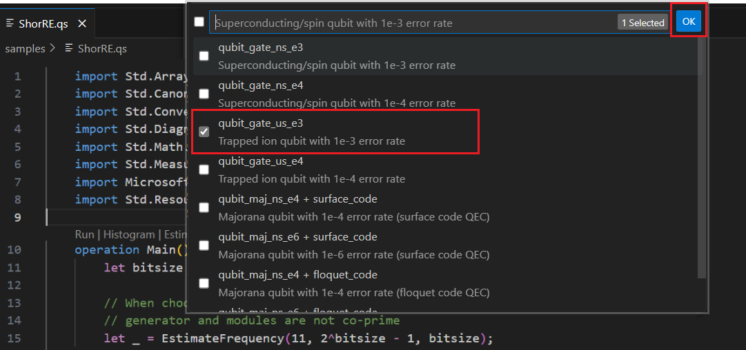
Resource Estimator には、6 つの定義済みの量子ビットパラメーターが用意されています。そのうちの 4 つにはゲートベースの命令セットがあり、2 つには Majorana 命令セットがあります。また、2 つの量子エラー修正コードと surface_code. floquet_code

この例では、qubit_gate_us_e3 量子ビットパラメーターと surface_code 量子エラー訂正コードを使って Resource Estimator を実行します。

[表示 -> コマンドパレット] を選択し、「リソース」と入力します。Q#: [リソース見積もりの計算] オプションが表示されます。また、操作の直前にMain] をクリックすることもできます。このオプションを選ぶと、Resource Estimator ウィンドウが開きます。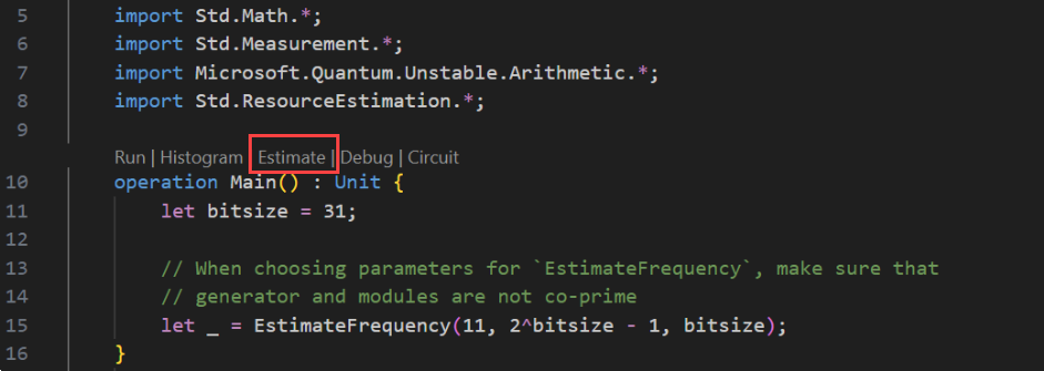
リソースを見積もる [量子ビットパラメーターとエラー訂正コード] の種類を 1 つまたは複数選ぶことができます。この例では、qubit_gate_us_e3 を選び、[OK] をクリックします。
[エラー予算] を指定するか、既定値の 0.001 を受け入れます。この例では、既定値のままにして Enter キーを押します。
ファイル名 (この場合は ShorRE) に基づいて既定の結果名をそのまま使用するには、Enter キーを押します。

結果の表示

Resource Estimator は、同じアルゴリズムに対して複数の見積もりを提供し、それぞれが量子ビット数とランタイムの間のトレードオフを示します。ランタイムとシステムスケールのトレードオフを理解することは、リソース推定の最も重要な側面の 1 つです。

リソース見積もりの結果は、[Q# 見積もり] ウィンドウに表示されます。

[結果] タブには、リソース見積もりの概要が表示されます。最初の行の横にあるアイコンをクリックして、表示する列を選びます。実行名、推定の種類、量子ビットの種類、qec スキーム、エラーバジェット、論理量子ビット、論理深さ、コード距離、T 状態、T ファクトリ、T ファクトリ分数、ランタイム、rQOPS、物理量子ビットから選択できます。

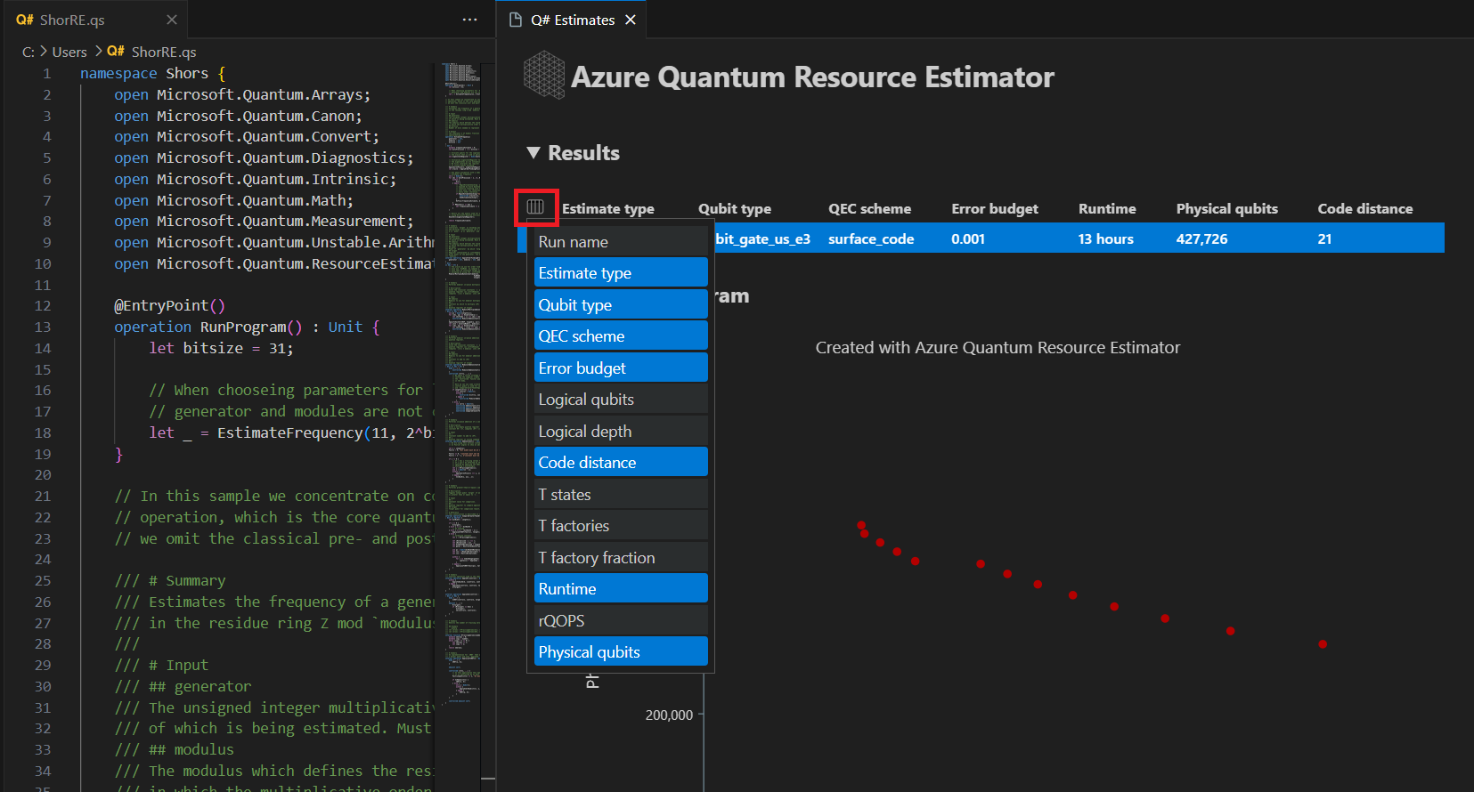
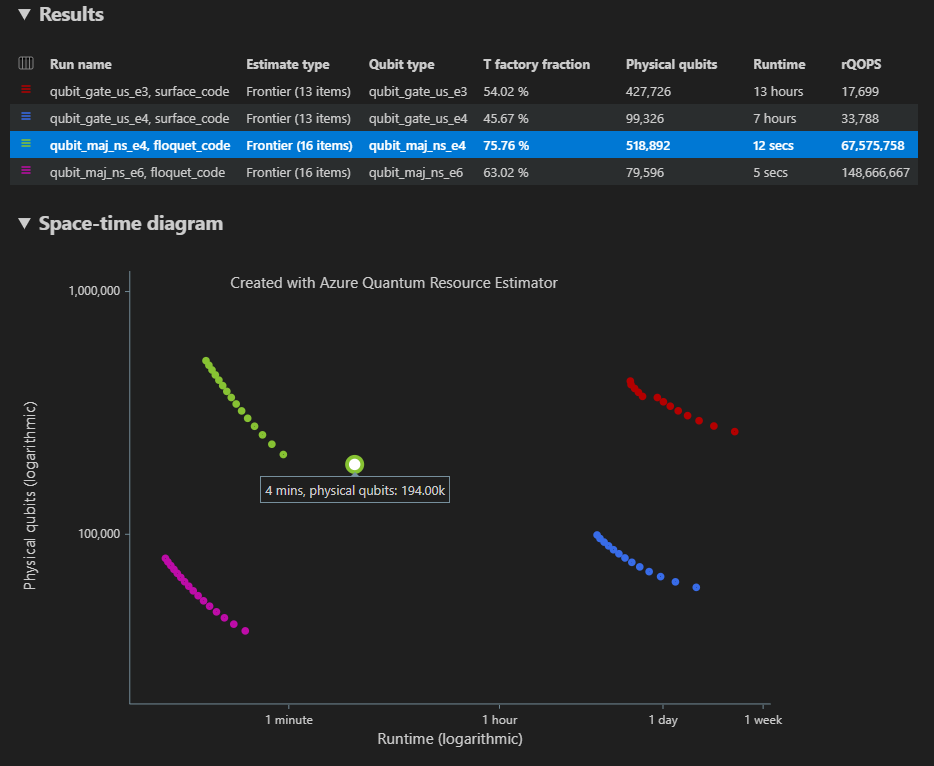
結果テーブルの [推定の種類] 列では、アルゴリズムの {量子ビット数、ランタイム} の最適な組み合わせの数を確認できます。これらの組み合わせは、時空間図で確認できます。
時空間図は、物理量子ビットの数とアルゴリズムのランタイムとのトレードオフを示しています。この場合、Resource Estimator は、数千の可能な組み合わせのうち、13 種類の最適な組み合わせを検出します。各 {量子ビット数、ランタイム} ポイントにカーソルを合わせると、その時点でのリソース推定の詳細を確認できます。

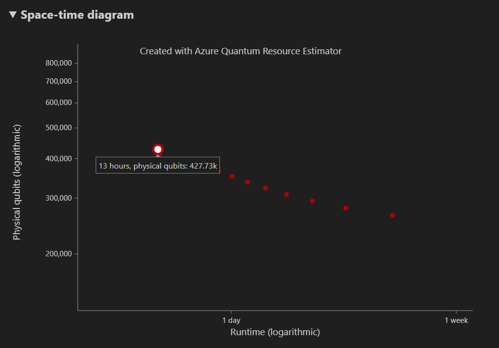
詳細については、時空間図を参照してください。

Note

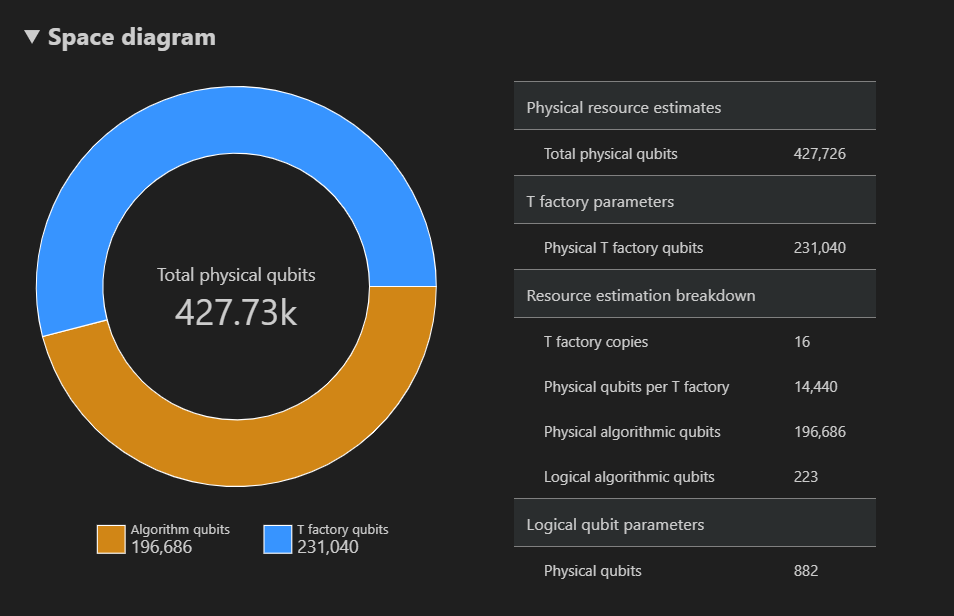
空間ダイアグラムとそのポイントに対応する リソース推定の詳細を表示するには、空間時間ダイアグラムの 1 つのポイント ({量子ビット数、ランタイム} ペア) をクリックする必要があります。
Space 図は、{number of qubits, runtime} ペアに対応する、アルゴリズムと T ファクトリに使用される物理量子ビットの分布を示しています。たとえば、時空間図で左端のポイントを選択した場合、アルゴリズムを実行するために必要な物理量子ビットの数は427726され、その196686はアルゴリズム量子ビット、そのうちの 231040 は T ファクトリ量子ビットです。

最後に、[リソース見積もり] タブには、{数量子ビット、ランタイム} ペアに対応するリソース推定器の出力データの完全な一覧が表示されます。詳しい情報が含まれているグループを折りたたんで、コストの詳細を確認できます。たとえば、時空間図の左端のポイントを選択し、[論理量子ビットパラメーター] グループを折りたたみます。

論理量子ビットパラメーター	Value
QEC スキーム	surface_code
コード距離	21
物理量子ビット	882
論理サイクル時間	13 ミリセクス
論理量子ビットエラー率	3.00E-13
交差の前因子	0.03
エラー訂正のしきい値	0.01
論理サイクル時間の数式	(4 * `twoQubitGateTime` + 2 * `oneQubitMeasurementTime`) * `codeDistance`
物理量子ビットの数式	2 * `codeDistance` * `codeDistance`

ヒント

[詳細行の表示] をクリックすると、レポートデータの各出力の説明が表示されます。

詳細については、リソース推定器の完全なレポートデータを参照してください。

パラメーターを変更するtarget

他の量子ビットの種類、エラー修正コード、およびエラー予算を使用して、同じ Q# プログラムのコストを見積もることができます。 [表示 - コマンドパレット>して[リソース推定]ウィンドウを開き、「」と入力します。Q#: Calculate Resource Estimates

Majorana ベースの量子ビットパラメーターなど、他の構成を選択します qubit_maj_ns_e6。既定のエラー予算値をそのまま使用するか、新しい予算値を入力して Enter キーを押します。リソース推定ツールは、新しい target パラメーターを使用して見積もりを再実行します。

詳細については、リソース推定器のパラメーターTarget

パラメーターの複数の構成を実行する

Azure Quantum Resource Estimator では、パラメーターの複数の target 構成を実行し、リソース推定結果を比較できます。

[表示 ] -> [コマンドパレット] を選択するか、Ctrl + Shift + P キーを押して「」と入力しますQ#: Calculate Resource Estimates。
qubit_gate_us_e3、qubit_gate_us_e4、qubit_maj_ns_e4 + floquet_code、およびqubit_maj_ns_e6 + floquet_codeを選択し、[OK] をクリックします。
既定のエラー予算値 0.001 をそのまま使用し、Enter キーを押します。
Enter キーを押して入力ファイル (この場合は ShorRE.qs) を受け入れます。
パラメーターが複数構成されている場合、結果は [結果] タブに異なる行に表示されます。
時空間図は、パラメーターのすべての構成の結果を示しています。結果テーブルの最初の列には、パラメーターの各構成の凡例が表示されます。各ポイントにカーソルを合わせると、その時点のリソース推定の詳細を確認できます。
時空間図の {number of qubits, runtime} ポイント をクリックして、対応する空間図とレポートデータを表示します。

VS Code での Jupyter Notebook の前提条件

Python と Pip がインストールされた Python 環境。
最新バージョンの Visual Studio Code または VS Code on the Web を開きます。
VS Code (Quantum 開発キット、Python、Jupyter 拡張機能をインストール)。

最新の Azure Quantum qsharp と qsharp_widgets パッケージ。

python -m pip install --upgrade qsharp qsharp_widgets

または

!pip install --upgrade qsharp qsharp_widgets

ヒント

Resource Estimator を実行するために Azure アカウントを持っている必要はありません。

量子アルゴリズムを作成する

VS Code で、[表示] > [コマンドパレット] を選択して、[作成: 新しい Jupyter Notebook] を選択します。
右上の VS Code は、Python のバージョンと、ノートブック用に選択された仮想 Python 環境を検出して表示します。複数の Python 環境がある場合は、右上のカーネルピッカーを使用してカーネルを選択する必要があります。環境が検出されなかった場合は、セットアップ情報については VS Code の Jupyter Notebook を参照してください。
ノートブックの最初のセルで、qsharp パッケージをインポートします。
```
import qsharp
```

新しいセルを追加して次のコードをコピーします。

%%qsharp
import Std.Arrays.*;
import Std.Canon.*;
import Std.Convert.*;
import Std.Diagnostics.*;
import Std.Math.*;
import Std.Measurement.*;
import Microsoft.Quantum.Unstable.Arithmetic.*;
import Std.ResourceEstimation.*;

operation RunProgram() : Unit {
    let bitsize = 31;

    // When choosing parameters for `EstimateFrequency`, make sure that
    // generator and modules are not co-prime
    let _ = EstimateFrequency(11, 2^bitsize - 1, bitsize);
}


// In this sample we concentrate on costing the `EstimateFrequency`
// operation, which is the core quantum operation in Shors algorithm, and
// we omit the classical pre- and post-processing.

/// # Summary
/// Estimates the frequency of a generator
/// in the residue ring Z mod `modulus`.
///
/// # Input
/// ## generator
/// The unsigned integer multiplicative order (period)
/// of which is being estimated. Must be co-prime to `modulus`.
/// ## modulus
/// The modulus which defines the residue ring Z mod `modulus`
/// in which the multiplicative order of `generator` is being estimated.
/// ## bitsize
/// Number of bits needed to represent the modulus.
///
/// # Output
/// The numerator k of dyadic fraction k/2^bitsPrecision
/// approximating s/r.
operation EstimateFrequency(
    generator : Int,
    modulus : Int,
    bitsize : Int
)
: Int {
    mutable frequencyEstimate = 0;
    let bitsPrecision =  2 * bitsize + 1;

    // Allocate qubits for the superposition of eigenstates of
    // the oracle that is used in period finding.
    use eigenstateRegister = Qubit[bitsize];

    // Initialize eigenstateRegister to 1, which is a superposition of
    // the eigenstates we are estimating the phases of.
    // We first interpret the register as encoding an unsigned integer
    // in little endian encoding.
    ApplyXorInPlace(1, eigenstateRegister);
    let oracle = ApplyOrderFindingOracle(generator, modulus, _, _);

    // Use phase estimation with a semiclassical Fourier transform to
    // estimate the frequency.
    use c = Qubit();
    for idx in bitsPrecision - 1..-1..0 {
        within {
            H(c);
        } apply {
            // `BeginEstimateCaching` and `EndEstimateCaching` are the operations
            // exposed by Azure Quantum Resource Estimator. These will instruct
            // resource counting such that the if-block will be executed
            // only once, its resources will be cached, and appended in
            // every other iteration.
            if BeginEstimateCaching("ControlledOracle", SingleVariant()) {
                Controlled oracle([c], (1 <<< idx, eigenstateRegister));
                EndEstimateCaching();
            }
            R1Frac(frequencyEstimate, bitsPrecision - 1 - idx, c);
        }
        if MResetZ(c) == One {
            frequencyEstimate += 1 <<< (bitsPrecision - 1 - idx);
        }
    }

    // Return all the qubits used for oracle eigenstate back to 0 state
    // using Microsoft.Quantum.Intrinsic.ResetAll.
    ResetAll(eigenstateRegister);

    return frequencyEstimate;
}

/// # Summary
/// Interprets `target` as encoding unsigned little-endian integer k
/// and performs transformation |k⟩ ↦ |gᵖ⋅k mod N ⟩ where
/// p is `power`, g is `generator` and N is `modulus`.
///
/// # Input
/// ## generator
/// The unsigned integer multiplicative order ( period )
/// of which is being estimated. Must be co-prime to `modulus`.
/// ## modulus
/// The modulus which defines the residue ring Z mod `modulus`
/// in which the multiplicative order of `generator` is being estimated.
/// ## power
/// Power of `generator` by which `target` is multiplied.
/// ## target
/// Register interpreted as little endian encoded which is multiplied by
/// given power of the generator. The multiplication is performed modulo
/// `modulus`.
internal operation ApplyOrderFindingOracle(
    generator : Int, modulus : Int, power : Int, target : Qubit[]
)
: Unit
is Adj + Ctl {
    // The oracle we use for order finding implements |x⟩ ↦ |x⋅a mod N⟩. We
    // also use `ExpModI` to compute a by which x must be multiplied. Also
    // note that we interpret target as unsigned integer in little-endian
    // encoding.
    ModularMultiplyByConstant(modulus,
                                ExpModI(generator, power, modulus),
                                target);
}

/// # Summary
/// Performs modular in-place multiplication by a classical constant.
///
/// # Description
/// Given the classical constants `c` and `modulus`, and an input
/// quantum register |𝑦⟩, this operation
/// computes `(c*x) % modulus` into |𝑦⟩.
///
/// # Input
/// ## modulus
/// Modulus to use for modular multiplication
/// ## c
/// Constant by which to multiply |𝑦⟩
/// ## y
/// Quantum register of target
internal operation ModularMultiplyByConstant(modulus : Int, c : Int, y : Qubit[])
: Unit is Adj + Ctl {
    use qs = Qubit[Length(y)];
    for (idx, yq) in Enumerated(y) {
        let shiftedC = (c <<< idx) % modulus;
        Controlled ModularAddConstant([yq], (modulus, shiftedC, qs));
    }
    ApplyToEachCA(SWAP, Zipped(y, qs));
    let invC = InverseModI(c, modulus);
    for (idx, yq) in Enumerated(y) {
        let shiftedC = (invC <<< idx) % modulus;
        Controlled ModularAddConstant([yq], (modulus, modulus - shiftedC, qs));
    }
}

/// # Summary
/// Performs modular in-place addition of a classical constant into a
/// quantum register.
///
/// # Description
/// Given the classical constants `c` and `modulus`, and an input
/// quantum register  |𝑦⟩, this operation
/// computes `(x+c) % modulus` into |𝑦⟩.
///
/// # Input
/// ## modulus
/// Modulus to use for modular addition
/// ## c
/// Constant to add to |𝑦⟩
/// ## y
/// Quantum register of target
internal operation ModularAddConstant(modulus : Int, c : Int, y : Qubit[])
: Unit is Adj + Ctl {
    body (...) {
        Controlled ModularAddConstant([], (modulus, c, y));
    }
    controlled (ctrls, ...) {
        // We apply a custom strategy to control this operation instead of
        // letting the compiler create the controlled variant for us in which
        // the `Controlled` functor would be distributed over each operation
        // in the body.
        //
        // Here we can use some scratch memory to save ensure that at most one
        // control qubit is used for costly operations such as `AddConstant`
        // and `CompareGreaterThenOrEqualConstant`.
        if Length(ctrls) >= 2 {
            use control = Qubit();
            within {
                Controlled X(ctrls, control);
            } apply {
                Controlled ModularAddConstant([control], (modulus, c, y));
            }
        } else {
            use carry = Qubit();
            Controlled AddConstant(ctrls, (c, y + [carry]));
            Controlled Adjoint AddConstant(ctrls, (modulus, y + [carry]));
            Controlled AddConstant([carry], (modulus, y));
            Controlled CompareGreaterThanOrEqualConstant(ctrls, (c, y, carry));
        }
    }
}

/// # Summary
/// Performs in-place addition of a constant into a quantum register.
///
/// # Description
/// Given a non-empty quantum register |𝑦⟩ of length 𝑛+1 and a positive
/// constant 𝑐 < 2ⁿ, computes |𝑦 + c⟩ into |𝑦⟩.
///
/// # Input
/// ## c
/// Constant number to add to |𝑦⟩.
/// ## y
/// Quantum register of second summand and target; must not be empty.
internal operation AddConstant(c : Int, y : Qubit[]) : Unit is Adj + Ctl {
    // We are using this version instead of the library version that is based
    // on Fourier angles to show an advantage of sparse simulation in this sample.

    let n = Length(y);
    Fact(n > 0, "Bit width must be at least 1");

    Fact(c >= 0, "constant must not be negative");
    Fact(c < 2 ^ n, $"constant must be smaller than {2L ^ n}");

    if c != 0 {
        // If c has j trailing zeroes than the j least significant bits
        // of y will not be affected by the addition and can therefore be
        // ignored by applying the addition only to the other qubits and
        // shifting c accordingly.
        let j = NTrailingZeroes(c);
        use x = Qubit[n - j];
        within {
            ApplyXorInPlace(c >>> j, x);
        } apply {
            IncByLE(x, y[j...]);
        }
    }
}

/// # Summary
/// Performs greater-than-or-equals comparison to a constant.
///
/// # Description
/// Toggles output qubit `target` if and only if input register `x`
/// is greater than or equal to `c`.
///
/// # Input
/// ## c
/// Constant value for comparison.
/// ## x
/// Quantum register to compare against.
/// ## target
/// Target qubit for comparison result.
///
/// # Reference
/// This construction is described in [Lemma 3, arXiv:2201.10200]
internal operation CompareGreaterThanOrEqualConstant(c : Int, x : Qubit[], target : Qubit)
: Unit is Adj+Ctl {
    let bitWidth = Length(x);

    if c == 0 {
        X(target);
    } elif c >= 2 ^ bitWidth {
        // do nothing
    } elif c == 2 ^ (bitWidth - 1) {
        ApplyLowTCNOT(Tail(x), target);
    } else {
        // normalize constant
        let l = NTrailingZeroes(c);

        let cNormalized = c >>> l;
        let xNormalized = x[l...];
        let bitWidthNormalized = Length(xNormalized);
        let gates = Rest(IntAsBoolArray(cNormalized, bitWidthNormalized));

        use qs = Qubit[bitWidthNormalized - 1];
        let cs1 = [Head(xNormalized)] + Most(qs);
        let cs2 = Rest(xNormalized);

        within {
            for i in IndexRange(gates) {
                (gates[i] ? ApplyAnd | ApplyOr)(cs1[i], cs2[i], qs[i]);
            }
        } apply {
            ApplyLowTCNOT(Tail(qs), target);
        }
    }
}

/// # Summary
/// Internal operation used in the implementation of GreaterThanOrEqualConstant.
internal operation ApplyOr(control1 : Qubit, control2 : Qubit, target : Qubit) : Unit is Adj {
    within {
        ApplyToEachA(X, [control1, control2]);
    } apply {
        ApplyAnd(control1, control2, target);
        X(target);
    }
}

internal operation ApplyAnd(control1 : Qubit, control2 : Qubit, target : Qubit)
: Unit is Adj {
    body (...) {
        CCNOT(control1, control2, target);
    }
    adjoint (...) {
        H(target);
        if (M(target) == One) {
            X(target);
            CZ(control1, control2);
        }
    }
}


/// # Summary
/// Returns the number of trailing zeroes of a number
///
/// ## Example
/// ```qsharp
/// let zeroes = NTrailingZeroes(21); // = NTrailingZeroes(0b1101) = 0
/// let zeroes = NTrailingZeroes(20); // = NTrailingZeroes(0b1100) = 2
/// ```
internal function NTrailingZeroes(number : Int) : Int {
    mutable nZeroes = 0;
    mutable copy = number;
    while (copy % 2 == 0) {
        nZeroes += 1;
        copy /= 2;
    }
    return nZeroes;
}

/// # Summary
/// An implementation for `CNOT` that when controlled using a single control uses
/// a helper qubit and uses `ApplyAnd` to reduce the T-count to 4 instead of 7.
internal operation ApplyLowTCNOT(a : Qubit, b : Qubit) : Unit is Adj+Ctl {
    body (...) {
        CNOT(a, b);
    }

    adjoint self;

    controlled (ctls, ...) {
        // In this application this operation is used in a way that
        // it is controlled by at most one qubit.
        Fact(Length(ctls) <= 1, "At most one control line allowed");

        if IsEmpty(ctls) {
            CNOT(a, b);
        } else {
            use q = Qubit();
            within {
                ApplyAnd(Head(ctls), a, q);
            } apply {
                CNOT(q, b);
            }
        }
    }

    controlled adjoint self;
}

量子アルゴリズムを見積もる

次に、既定の前提条件を使用して RunProgram 操作の物理リソースを推定します。新しいセルを追加して次のコードをコピーします。

result = qsharp.estimate("RunProgram()")
result

qsharp.estimate 関数は結果オブジェクトを作成し、これは全体的な物理リソースの総数を含むテーブルを表示するために使用できます。詳しい情報が含まれているグループを展開して、コストの詳細を確認できます。詳細については、リソース推定器の完全なレポートデータを参照してください。

たとえば、論理量子ビットパラメーター グループを展開すると、コード距離が 21 で、物理量子ビットの数が 882 であることがわかります。

論理量子ビットパラメーター	Value
QEC スキーム	surface_code
コード距離	21
物理量子ビット	882
論理サイクル時間	8 ミリセクス
論理量子ビットエラー率	3.00E-13
交差の前因子	0.03
エラー訂正のしきい値	0.01
論理サイクル時間の数式	(4 * `twoQubitGateTime` + 2 * `oneQubitMeasurementTime`) * `codeDistance`
物理量子ビットの数式	2 * `codeDistance` * `codeDistance`

ヒント

よりコンパクトなバージョンの出力テーブルが必要であれば、result.summary を使用できます。

空間図

アルゴリズムと T ファクトリに使用される物理量子ビットの分布は、アルゴリズムの設計に影響を与える可能性のある要因です。 qsharp-widgets パッケージを使用してこの分布を視覚化すると、アルゴリズムの推定される空間的要件をより深く理解できます。

from qsharp-widgets import SpaceChart, EstimateDetails
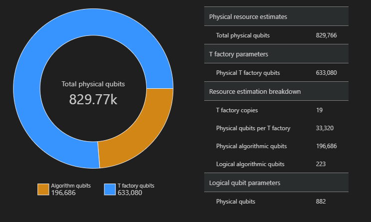
SpaceChart(result)

この例では、アルゴリズムを実行するために必要な物理量子ビットの数は 829766 であり、そのうちの 196686 個がアルゴリズム量子ビットであり、633080 個が T ファクトリ量子ビットです。

リソース推定器の空間図を示すスクリーンショット。

既定値を変更し、アルゴリズムの見積もりを行う

プログラムのリソース見積もり要求を送信する際には、いくつかのオプションのパラメーターを指定できます。このフィールドを jobParams 使用して、 target ジョブの実行に渡すことができるすべてのパラメーターにアクセスし、想定された既定値を確認します。

result['jobParams']

{'errorBudget': 0.001,
 'qecScheme': {'crossingPrefactor': 0.03,
  'errorCorrectionThreshold': 0.01,
  'logicalCycleTime': '(4 * twoQubitGateTime + 2 * oneQubitMeasurementTime) * codeDistance',
  'name': 'surface_code',
  'physicalQubitsPerLogicalQubit': '2 * codeDistance * codeDistance'},
 'qubitParams': {'instructionSet': 'GateBased',
  'name': 'qubit_gate_ns_e3',
  'oneQubitGateErrorRate': 0.001,
  'oneQubitGateTime': '50 ns',
  'oneQubitMeasurementErrorRate': 0.001,
  'oneQubitMeasurementTime': '100 ns',
  'tGateErrorRate': 0.001,
  'tGateTime': '50 ns',
  'twoQubitGateErrorRate': 0.001,
  'twoQubitGateTime': '50 ns'}}

Resource Estimator は、見積もりの既定値として、qubit_gate_ns_e3 量子ビットモデル、surface_code 誤り訂正符号、および 0.001 のエラーバジェットを使用することがわかります。

targetカスタマイズできるパラメーターは次のとおりです。

errorBudget - アルゴリズムで許容される合計のエラーバジェット
qecScheme - 量子誤り訂正 (QEC) スキーム
qubitParams - 物理量子ビットパラメーター
constraints - コンポーネントレベルの制約
distillationUnitSpecifications - T ファクトリ蒸留アルゴリズムに対する指定
estimateType - シングルまたはフロンティア

詳細については、リソース推定器のパラメーターTarget

量子ビットモデルを変更する

Majorana ベースの量子ビットパラメーター (qubitParams) "qubit_maj_ns_e6" を使用して、同じアルゴリズムのコストを見積もることができます。

result_maj = qsharp.estimate("RunProgram()", params={
                "qubitParams": {
                    "name": "qubit_maj_ns_e6"
                }})
EstimateDetails(result_maj)

量子誤り訂正スキームを変更する

floqued QEC スキーム qecScheme を使用して、Majorana ベースの量子ビットパラメーターで同じ例のリソース見積もりジョブを再実行できます。

result_maj = qsharp.estimate("RunProgram()", params={
                "qubitParams": {
                    "name": "qubit_maj_ns_e6"
                },
                "qecScheme": {
                    "name": "floquet_code"
                }})
EstimateDetails(result_maj)

エラーバジェットを変更する

次に、10% の errorBudget で同じ量子回路を再実行します。

result_maj = qsharp.estimate("RunProgram()", params={
                "qubitParams": {
                    "name": "qubit_maj_ns_e6"
                },
                "qecScheme": {
                    "name": "floquet_code"
                },
                "errorBudget": 0.1})
EstimateDetails(result_maj)

リソース推定機能を使用したバッチ処理

Azure Quantum Resource Estimator を使用すると、パラメーターの複数の target 構成を実行し、結果を比較できます。これはさまざまな量子ビットモデル、QEC スキーム、またはエラーバジェットのコストを比較したい場合に便利です。

パラメーターの一覧を関数の target パラメーターに渡すことで、 params バッチ推定を qsharp.estimate 実行できます。たとえば、既定のパラメーターを使用して同じアルゴリズムを実行し、フローケ QEC スキームを使用して Majorana ベースの量子ビットパラメーターを実行します。

result_batch = qsharp.estimate("RunProgram()", params=
                [{}, # Default parameters
                {
                    "qubitParams": {
                        "name": "qubit_maj_ns_e6"
                    },
                    "qecScheme": {
                        "name": "floquet_code"
                    }
                }])
result_batch.summary_data_frame(labels=["Gate-based ns, 10⁻³", "Majorana ns, 10⁻⁶"])

モデル	論理量子ビット	論理的な深さ	T 状態	コード距離	T ファクトリ	T ファクトリ小数	物理量子ビット	rQOPS	物理ランタイム
ゲートベースの ns、10⁻³	223	3.64M	4.70M	21	19	76.30 %	829.77k	26.55M	31 秒
Majorana の ns、10⁻⁶	223	3.64M	4.70M	5	19	63.02 %	79.60k	148.67M	5 秒

クラスEstimatorParams作成することもできます。

from qsharp.estimator import EstimatorParams, QubitParams, QECScheme, LogicalCounts

labels = ["Gate-based µs, 10⁻³", "Gate-based µs, 10⁻⁴", "Gate-based ns, 10⁻³", "Gate-based ns, 10⁻⁴", "Majorana ns, 10⁻⁴", "Majorana ns, 10⁻⁶"]

params = EstimatorParams(num_items=6)
params.error_budget = 0.333
params.items[0].qubit_params.name = QubitParams.GATE_US_E3
params.items[1].qubit_params.name = QubitParams.GATE_US_E4
params.items[2].qubit_params.name = QubitParams.GATE_NS_E3
params.items[3].qubit_params.name = QubitParams.GATE_NS_E4
params.items[4].qubit_params.name = QubitParams.MAJ_NS_E4
params.items[4].qec_scheme.name = QECScheme.FLOQUET_CODE
params.items[5].qubit_params.name = QubitParams.MAJ_NS_E6
params.items[5].qec_scheme.name = QECScheme.FLOQUET_CODE

qsharp.estimate("RunProgram()", params=params).summary_data_frame(labels=labels)

モデル	論理量子ビット	論理的な深さ	T 状態	コード距離	T ファクトリ	T ファクトリ小数	物理量子ビット	rQOPS	物理ランタイム
ゲートベースの µs、10⁻³	223 3.64M	4.70M	17	13	40.54 %	216.77k	21.86k	10 時間
ゲートベースの µs、10⁻⁴	223	3.64M	4.70M	9	14	43.17 %	63.57k	41.30k	5 時間
ゲートベースの ns、10⁻³	223 3.64M	4.70M	17	16	69.08 %	416.89k	32.79M	25 秒
ゲートベースの ns、10⁻⁴	223 3.64M	4.70M	9	14	43.17 %	63.57k	61.94M	13 秒
Majorana の ns、10⁻⁴	223 3.64M	4.70M	9	19	82.75 %	501.48k	82.59M	10 秒
Majorana の ns、10⁻⁶	223 3.64M	4.70M	5	13	31.47 %	42.96k	148.67M	5 秒

パレートフロンティア推定の実行

アルゴリズムのリソースを推定するときは、物理量子ビットの数とアルゴリズムのランタイムとのトレードオフを考慮することが重要です。アルゴリズムの実行時間を短縮するために、可能な限り多くの物理量子ビットの割り当てを検討できます。ただし、物理量子ビットの数は、量子ハードウェアで使用可能な物理量子ビットの数によって制限されます。

パレートフロンティア推定は、同じアルゴリズムに対して複数の推定値を提供し、それぞれが量子ビット数とランタイムの間のトレードオフを持ちます。

パレートフロンティア推定を使用してリソース推定を実行するには、パラメーター"estimateType"を target"frontier" . たとえば、パレートフロンティア推定を使用して、サーフェスコードを使用して、Majorana ベースの量子ビットパラメーターで同じアルゴリズムを実行します。
```
result = qsharp.estimate("RunProgram()", params=
                            {"qubitParams": { "name": "qubit_maj_ns_e4" },
                            "qecScheme": { "name": "surface_code" },
                            "estimateType": "frontier", # frontier estimation
                            }
                        )
```
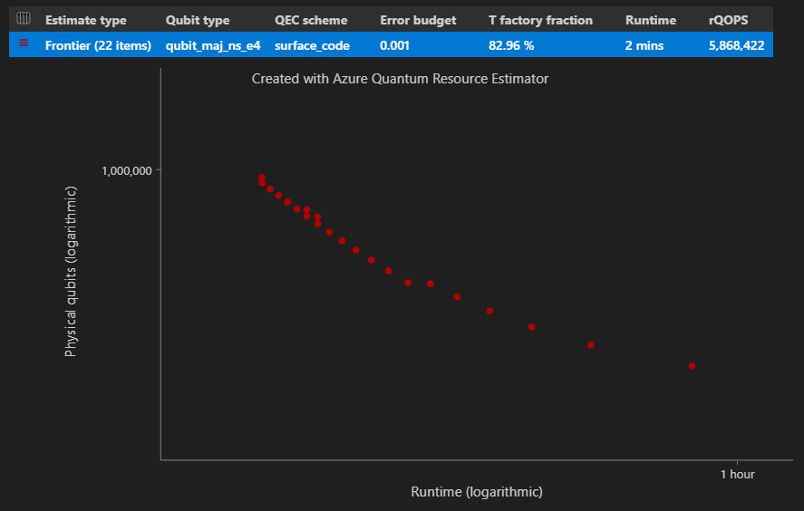
この関数を EstimatesOverview 使用すると、物理リソースの合計数全体を含むテーブルを表示できます。最初の行の横にあるアイコンをクリックして、表示する列を選びます。実行名、推定の種類、量子ビットの種類、qec スキーム、エラーバジェット、論理量子ビット、論理深さ、コード距離、T 状態、T ファクトリ、T ファクトリ分数、ランタイム、rQOPS、物理量子ビットから選択できます。
```
from qsharp_widgets import EstimatesOverview
EstimatesOverview(result)
```

結果テーブルの [推定の種類 ] 列では、アルゴリズムの {量子ビット数、ランタイム} のさまざまな組み合わせの数を確認できます。この場合、Resource Estimator は、可能な数千の組み合わせのうち、22 種類の最適な組み合わせを検出します。

時空間図

この関数には EstimatesOverview 、リソース推定器の時空間図も表示されます。

時空間図は、物理量子ビットの数と、各 {量子ビット数、ランタイム} ペアのアルゴリズムのランタイムを示しています。各ポイントにカーソルを合わせると、その時点のリソース推定の詳細を確認できます。

リソース推定機能のフロンティア推定を含む時空間図を示すスクリーンショット。

パレートフロンティア推定によるバッチ処理

パラメーターの複数の target 構成をフロンティア推定と推定して比較するには、パラメーターを追加 "estimateType": "frontier", します。

result = qsharp.estimate(
    "RunProgram()",
    [
        {
        "qubitParams": { "name": "qubit_maj_ns_e4" },
        "qecScheme": { "name": "surface_code" },
        "estimateType": "frontier", # Pareto frontier estimation
        },
        {
        "qubitParams": { "name": "qubit_maj_ns_e6" },
        "qecScheme": { "name": "floquet_code" },
        "estimateType": "frontier", # Pareto frontier estimation
        },
    ]
)

EstimatesOverview(result, colors=["#1f77b4", "#ff7f0e"], runNames=["e4 Surface Code", "e6 Floquet Code"])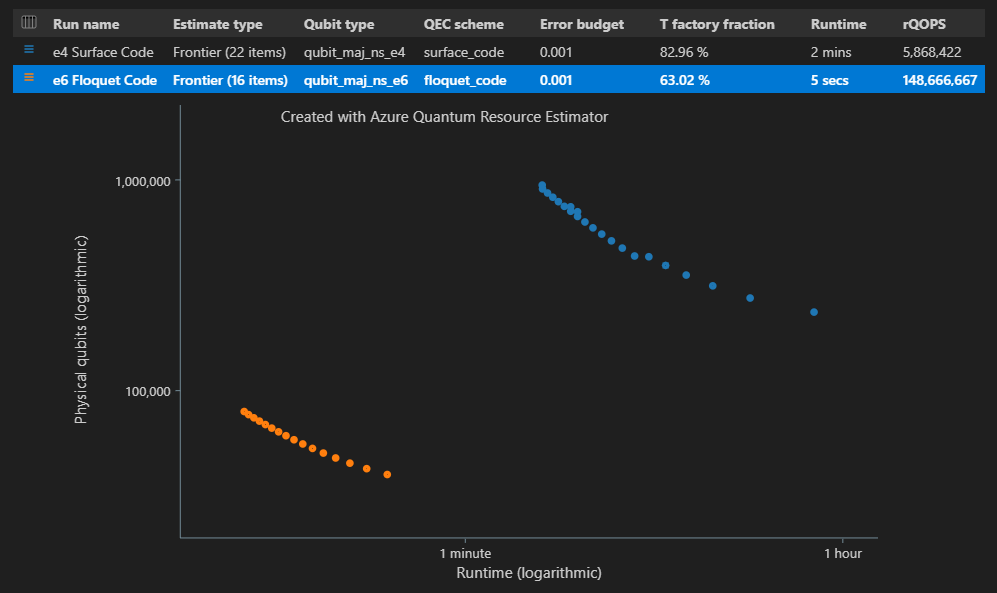

パラメーターのパレートフロンティア推定と複数の構成を使用する場合のリソース推定器の時空間図を示すスクリーンショット。

Note

関数を使用して、量子ビット時間ダイアグラムの色と実行名を EstimatesOverview 定義できます。

パレートフロンティア推定を使用して複数の target パラメーター構成を実行すると、時空間図の特定のポイント ({量子ビット数、ランタイム} ペア) のリソース推定値を確認できます。たとえば、次のコードは、2 番目の実行 (推定インデックス = 0) と 4 番目の (ポイントインデックス = 3) 最短ランタイムの推定詳細の使用状況を示しています。
```
EstimateDetails(result[1], 4)
```
また、空間図の特定のポイントの空間図を確認することもできます。たとえば、次のコードは、組み合わせの最初の実行 (推定インデックス = 0) と 3 番目に短いランタイム (ポイントインデックス = 2) のスペース図を示しています。
```
SpaceChart(result[0], 2)
```

VS Code での Qiskit の前提条件

Python と Pip がインストールされた Python 環境。
最新バージョンの Visual Studio Code を使用するか、Web 上で Visual Studio Code を開きます。
VS Code (Quantum 開発キット、Python、Jupyter 拡張機能をインストール)。

最新の Azure Quantum の qsharp、qsharp_widgets、および qiskit パッケージ。

python -m pip install --upgrade qsharp qsharp_widgets qiskit

または

!pip install --upgrade qsharp qsharp_widgets qiskit

ヒント

Resource Estimator を実行するために Azure アカウントを持っている必要はありません。

新しい Jupyter Notebook を作成する

VS Code で、[表示] > [コマンドパレット] を選択して、[作成: 新しい Jupyter Notebook] を選択します。
右上の VS Code は、Python のバージョンと、ノートブック用に選択された仮想 Python 環境を検出して表示します。複数の Python 環境がある場合は、右上のカーネルピッカーを使用してカーネルを選択する必要があります。環境が検出されなかった場合は、セットアップ情報については VS Code の Jupyter Notebook を参照してください。

量子アルゴリズムを作成する

この例では、クォンタムフーリエ変換を使用して算術演算を実装する、Ruiz-Perez と Garcia-Escartin (arXiv:1411.5949) で提示される構成に基づいて、乗数の量子回路を作成します。

変数を変更することで、乗数のサイズを bitwidth 調整できます。回路生成は、乗数の値で bitwidth 呼び出すことができる関数にラップされます。この操作には、指定されたサイズの 2 つの入力レジスタと、指定した bitwidthサイズの 2 倍の 1 つの出力レジスタがあります bitwidth。また、この関数は、量子回路から直接抽出された乗数の論理リソース数も出力します。

from qiskit.circuit.library import RGQFTMultiplier 

def create_algorithm(bitwidth):
    print(f"[INFO] Create a QFT-based multiplier with bitwidth {bitwidth}")

    circ = RGQFTMultiplier(num_state_qubits=bitwidth)

    return circ

Note

Python カーネルを選択しても qiskit モジュールが認識されない場合は、カーネルピッカーで別の Python 環境を選択してみてください。

量子アルゴリズムを見積もる

関数を使用してアルゴリズムのインスタンスを create_algorithm 作成します。変数を変更することで、乗数のサイズを bitwidth 調整できます。

bitwidth = 4

circ = create_algorithm(bitwidth)

既定の前提条件を使用して、この操作の物理リソースを見積もります。 estimate 呼び出しを使用できます。このメソッドは、Qiskit から QuantumCircuit オブジェクトを受け取るためにオーバーロードされています。

from qsharp.estimator import EstimatorParams
from qsharp.interop.qiskit import estimate

params = EstimatorParams()
result = estimate(circ, params)

または、ResourceEstimatorBackend を使用して、既存のバックエンドと同様に見積もりを実行することもできます。

from qsharp.interop.qiskit import ResourceEstimatorBackend
from qsharp.estimator import EstimatorParams

params = EstimatorParams()
backend = ResourceEstimatorBackend()

job = backend.run(circ, params)
result = job.result()

result オブジェクトには、リソース推定ジョブの出力が含まれています。 EstimateDetails 関数を使用すると、結果をより読みやすい形式で表示できます。

from qsharp_widgets import EstimateDetails
EstimateDetails(result)

EstimateDetails 関数では、全体的な物理リソース数を含むテーブルが表示されます。詳しい情報が含まれているグループを展開して、コストの詳細を確認できます。詳細については、リソース推定器の完全なレポートデータを参照してください。

たとえば、論理量子ビットパラメーター グループを展開すると、エラー修正コードの距離が 15 であることがわかります。

論理量子ビットパラメーター	Value
QEC スキーム	surface_code
コード距離	15
物理量子ビット	450
論理サイクル時間	6us
論理量子ビットエラー率	3.00E-10
交差の前因子	0.03
エラー訂正のしきい値	0.01
論理サイクル時間の数式	(4 * `twoQubitGateTime` + 2 * `oneQubitMeasurementTime`) * `codeDistance`
物理量子ビットの数式	2 * `codeDistance` * `codeDistance`

[物理量子ビットパラメーター] グループでは、この推定で想定されていた物理量子ビットのプロパティを確認できます。たとえば、単一量子ビット測定と単一量子ビットゲートを実行する時間は、それぞれ 100 ns と 50 ns であると見なされます。

ヒント

result.data() メソッドを使用して、Python ディクショナリとして Resource Estimator の出力にアクセスすることもできます。たとえば、物理カウントにアクセスするには result.data()["physicalCounts"] のように指定します。

空間図

アルゴリズムと T ファクトリに使用される物理量子ビットの分布は、アルゴリズムの設計に影響を与える可能性のある要因です。この分布を視覚化して、アルゴリズムの推定領域要件をより深く理解できます。

from qsharp_widgets import SpaceChart

SpaceChart(result)

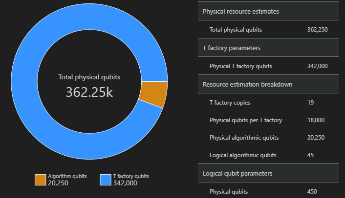
アルゴリズム量子ビットと T ファクトリ量子ビットの間の物理量子ビットの合計分布を示す円グラフ。T ファクトリのコピー数と T ファクトリあたりの物理量子ビット数の内訳を含むテーブルがあります。

空間図は、アルゴリズム量子ビットと T ファクトリ量子ビットの割合を示しています。 T ファクトリのコピーの数である 19 は、T ファクトリの物理量子ビットの数に寄与することに注意してください。式としては、T ファクトリの数に T ファクトリあたりの物理量子ビットをかけて 19 \cdot 18,000 = 342,000 となります。

詳細については、T ファクトリの物理見積もりを参照してください。

既定値を変更し、アルゴリズムの見積もりを行う

プログラムのリソース見積もり要求を送信する際には、いくつかのオプションのパラメーターを指定できます。このフィールドを jobParams 使用して、ジョブの実行に渡すことができるすべての値にアクセスし、想定されていた既定値を確認します。

result.data()["jobParams"]

{'errorBudget': 0.001,
 'qecScheme': {'crossingPrefactor': 0.03,
  'errorCorrectionThreshold': 0.01,
  'logicalCycleTime': '(4 * twoQubitGateTime + 2 * oneQubitMeasurementTime) * codeDistance',
  'name': 'surface_code',
  'physicalQubitsPerLogicalQubit': '2 * codeDistance * codeDistance'},
 'qubitParams': {'instructionSet': 'GateBased',
  'name': 'qubit_gate_ns_e3',
  'oneQubitGateErrorRate': 0.001,
  'oneQubitGateTime': '50 ns',
  'oneQubitMeasurementErrorRate': 0.001,
  'oneQubitMeasurementTime': '100 ns',
  'tGateErrorRate': 0.001,
  'tGateTime': '50 ns',
  'twoQubitGateErrorRate': 0.001,
  'twoQubitGateTime': '50 ns'}}

targetカスタマイズできるパラメーターは次のとおりです。

errorBudget - 許容される全体的なエラー予算
qecScheme - 量子誤り訂正 (QEC) スキーム
qubitParams - 物理量子ビットパラメーター
constraints - コンポーネントレベルの制約
distillationUnitSpecifications - T ファクトリ蒸留アルゴリズムに対する指定

詳細については、リソース推定器のパラメーターTarget

量子ビットモデルを変更する

次に、Majorana ベースの量子ビットパラメーターを使用して、同じアルゴリズムのコストを見積もります qubit_maj_ns_e6

qubitParams = {
    "name": "qubit_maj_ns_e6"
}

result = backend.run(circ, qubitParams).result()

プログラムを使用して、物理数を調べることができます。たとえば、アルゴリズムを実行するために作成された T ファクトリの詳細を調べることができます。

result.data()["tfactory"]

{'eccDistancePerRound': [1, 1, 5],
 'logicalErrorRate': 1.6833177305222897e-10,
 'moduleNamePerRound': ['15-to-1 space efficient physical',
  '15-to-1 RM prep physical',
  '15-to-1 RM prep logical'],
 'numInputTstates': 20520,
 'numModulesPerRound': [1368, 20, 1],
 'numRounds': 3,
 'numTstates': 1,
 'physicalQubits': 16416,
 'physicalQubitsPerRound': [12, 31, 1550],
 'runtime': 116900.0,
 'runtimePerRound': [4500.0, 2400.0, 110000.0]}

Note

既定では、ランタイムはナノ秒単位で表示されます。

このデータを使用して、T ファクトリが必要な T 状態を生成する方法に関するいくつかの説明を生成できます。

data = result.data()
tfactory = data["tfactory"]
breakdown = data["physicalCounts"]["breakdown"]
producedTstates = breakdown["numTfactories"] * breakdown["numTfactoryRuns"] * tfactory["numTstates"]

print(f"""A single T factory produces {tfactory["logicalErrorRate"]:.2e} T states with an error rate of (required T state error rate is {breakdown["requiredLogicalTstateErrorRate"]:.2e}).""")
print(f"""{breakdown["numTfactories"]} copie(s) of a T factory are executed {breakdown["numTfactoryRuns"]} time(s) to produce {producedTstates} T states ({breakdown["numTstates"]} are required by the algorithm).""")
print(f"""A single T factory is composed of {tfactory["numRounds"]} rounds of distillation:""")
for round in range(tfactory["numRounds"]):
    print(f"""- {tfactory["numUnitsPerRound"][round]} {tfactory["unitNamePerRound"][round]} unit(s)""")

A single T factory produces 1.68e-10 T states with an error rate of (required T state error rate is 2.77e-08).
23 copies of a T factory are executed 523 time(s) to produce 12029 T states (12017 are required by the algorithm).
A single T factory is composed of 3 rounds of distillation:
- 1368 15-to-1 space efficient physical unit(s)
- 20 15-to-1 RM prep physical unit(s)
- 1 15-to-1 RM prep logical unit(s)

量子誤り訂正スキームを変更する

次に、浮動 QEC スキーム qecSchemeを使用して、Majorana ベースの量子ビットパラメーターで同じ例のリソース推定ジョブを再実行します。

params = {
    "qubitParams": {"name": "qubit_maj_ns_e6"},
    "qecScheme": {"name": "floquet_code"}
}

result_maj_floquet = backend.run(circ, params).result()
EstimateDetails(result_maj_floquet)

エラーバジェットを変更する

10% の同じ量子回路を errorBudget 再実行してみましょう。

params = {
    "errorBudget": 0.01,
    "qubitParams": {"name": "qubit_maj_ns_e6"},
    "qecScheme": {"name": "floquet_code"},
}
result_maj_floquet_e1 = backend.run(circ, params).result()
EstimateDetails(result_maj_floquet_e1)

Note

リソース推定ツールの使用中に問題が発生した場合は、[トラブルシューティング] ページを確認するか、お問い合わせくださいAzureQuantumInfo@microsoft.com。

次の方法で共有

リソース推定ツールを実行するさまざまな方法

VS Code の前提条件

新しい Q# ファイルを作成する

量子アルゴリズムを作成する

Resource Estimator を実行する

結果の表示

パラメーターを変更するtarget

パラメーターの複数の構成を実行する

VS Code での Jupyter Notebook の前提条件

量子アルゴリズムを作成する

量子アルゴリズムを見積もる

空間図

既定値を変更し、アルゴリズムの見積もりを行う

量子ビットモデルを変更する

量子誤り訂正スキームを変更する

エラーバジェットを変更する

リソース推定機能を使用したバッチ処理

パレートフロンティア推定の実行

時空間図

パレートフロンティア推定によるバッチ処理

VS Code での Qiskit の前提条件

新しい Jupyter Notebook を作成する

量子アルゴリズムを作成する

量子アルゴリズムを見積もる

空間図

既定値を変更し、アルゴリズムの見積もりを行う

量子ビットモデルを変更する

量子誤り訂正スキームを変更する

エラーバジェットを変更する

次のステップ

フィードバック

その他のリソース

次の方法で共有

リソース推定ツールを実行するさまざまな方法

VS Code の前提条件

新しい Q# ファイルを作成する

量子アルゴリズムを作成する

Resource Estimator を実行する

結果の表示

パラメーターを変更するtarget

パラメーターの複数の構成を実行する

VS Code での Jupyter Notebook の前提条件

量子アルゴリズムを作成する

量子アルゴリズムを見積もる

空間図

既定値を変更し、アルゴリズムの見積もりを行う

量子ビット モデルを変更する

量子誤り訂正スキームを変更する

エラー バジェットを変更する

リソース推定機能を使用したバッチ処理

パレートフロンティア推定の実行

時空間図

パレートフロンティア推定によるバッチ処理

VS Code での Qiskit の前提条件

新しい Jupyter Notebook を作成する

量子アルゴリズムを作成する

量子アルゴリズムを見積もる

空間図

既定値を変更し、アルゴリズムの見積もりを行う

量子ビット モデルを変更する

量子誤り訂正スキームを変更する

エラー バジェットを変更する

次のステップ

フィードバック

その他のリソース

量子ビットモデルを変更する

エラーバジェットを変更する

量子ビットモデルを変更する

エラーバジェットを変更する