Forecast the impact of business practice changes on emissions
The AI-powered what-if analysis feature in Microsoft Sustainability Manager enables you to forecast the impact of business practice changes on your overall emissions footprint. What-if analysis is a custom AI model in Microsoft Sustainability Manager that allows you to compare your current carbon emissions trends against the forecasted carbon emissions impact, of changing variables in your business model. It helps you to create more informed carbon reduction strategies and accelerate your overall sustainability goals.
Using the what-if analysis tool, you can:
Customize AI modeling with your organization’s carbon activity data and return forecasts in mtCO2e.
Apply predefined scenarios tailored to your organization’s needs.
Supported scenarios
What-if analysis supports the following scenarios. Each scenario offers different levels of customizability, enabling you to tailor the forecast to your organization’s specific data and needs. The following table lists all the available variables for each data type.
| Scenario category | Available variables |
|---|---|
| Industrial process | - Cost - Goods quantity - Industrial process type - Spend type - Quantity |
| Mobile combustion | - Cost - Distance - Fuel quantity - Fuel type - Goods quantity - Industrial process type - Quantity - Spend type - Vehicle type |
| Stationary combustion | - Cost - Energy conversion ratio - Fuel quantity - Fuel type - Goods quantity - Industrial process type - Quantity - Spend type |
| Purchased cooling | - Contractual instrument type - Cost - Goods quantity - Is renewable - Quantity - Spend type |
| Purchased electricity | - Contractual instrument type - Cost - Goods quantity - Is renewable - Quantity - Spend type |
| Purchased heat | - Contractual instrument type - Cost - Goods quantity - Is renewable - Quantity - Spend type |
| Purchased steam | - Contractual instrument type - Cost - Goods quantity - Is renewable - Quantity - Spend type |
| 1. Purchased goods and services | - Cost - Goods quantity - Industrial process type - Quantity - Spend type |
| 2. Capital goods | - Cost - Industrial process type - Quantity - Spend type |
| 4. Upstream transportation and distribution | - Cost - Distance - Fuel quantity - Fuel type - Goods quantity - Industrial process type - Quantity - Spend type - Transport mode - Transportation and distribution type - Vehicle type |
| 5. Waste generated in operations | - Cost - Disposal method - Distance - Fuel quantity - Industrial process type - Material - Quantity - Spend type - Transport mode - Waste quantity |
| 6. Business travel | - Business travel type - Cost - Distance - Fuel quantity - Industrial process type - Quantity - Vehicle type |
| 7. Employee commuting | - Cost - Distance - Employee commuting type - Fuel quantity - Fuel type - Industrial process type - Quantity - Vehicle type |
| 9. Downstream transportation and distribution | - Cost - Distance - Fuel quantity - Fuel type - Goods quantity - Industrial process type - Quantity - Spend type - Transport mode - Transportation and distribution type - Vehicle type |
| 12. End-of-life treatment of sold products | - Cost - Disposal method - Distance - Fuel quantity - Industrial process type - Material - Quantity - Spend type - Transport mode |
Forecast scenario: Important considerations
Keep these considerations in mind while creating your forecast scenario.
You can layer between one and three strategies within a single scenario using the Number of scenarios field.
The Variable(s) field is multi-select, enabling you to choose the data or quantities you wish to forecast changes for. For example, you can choose to modify the Cost, Distance, and Goods quantity being transported as part of your 4. Upstream transportation and distribution scenario.
Every scenario requires the following fields:
Name
Organizational unit
Data type
Calculation model
AR version
Number of strategies
Variable(s)
Facility isn't required for every scenario, but you can use it to further narrow down the data for your forecast.
Supported time series forecasting models
Sustainability Manager supports (Seasonal) Auto Regressive Integrated Moving Average (S)ARIMA) and Error Trend Seasonality (ETS) univariate time series forecasting models for generating forecasts on activity data. ETS models rely on the descriptions of trend and seasonality in the data, while ARIMA models describe the autocorrelations in the data.
The model selection framework chooses the best forecasting model based on historical activity data. The generated activity-level forecasts are then processed through the calculation model to convert them into emissions-level forecasts. In cases where the historical data is insufficient or highly irregular, a simpler fallback model is used instead of ARIMA or ETS.
To learn more about these models, refer to Chapter 7 (Exponential Smoothing) and Chapter 8 (ARIMA models) of the Forecasting: Principles and Practice textbook.
Solution focus area
Personas and scenarios
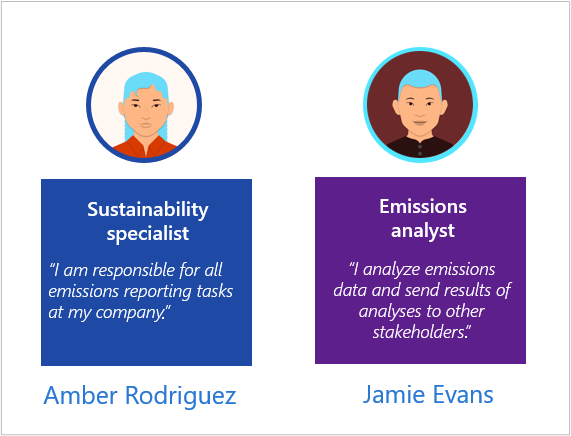
Let us consider the following fictional personas for the scenarios of Contoso APAC and Contoso Pod Business:
Amber Rodriguez - Sustainability specialist
Jamie Evans - Emissions analyst
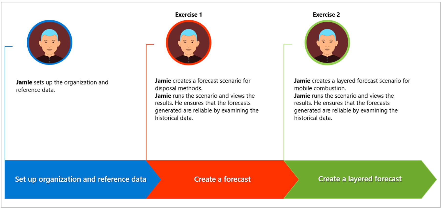
These personas participate in the following sequential scenarios:
Scenario 1: Create a forecast
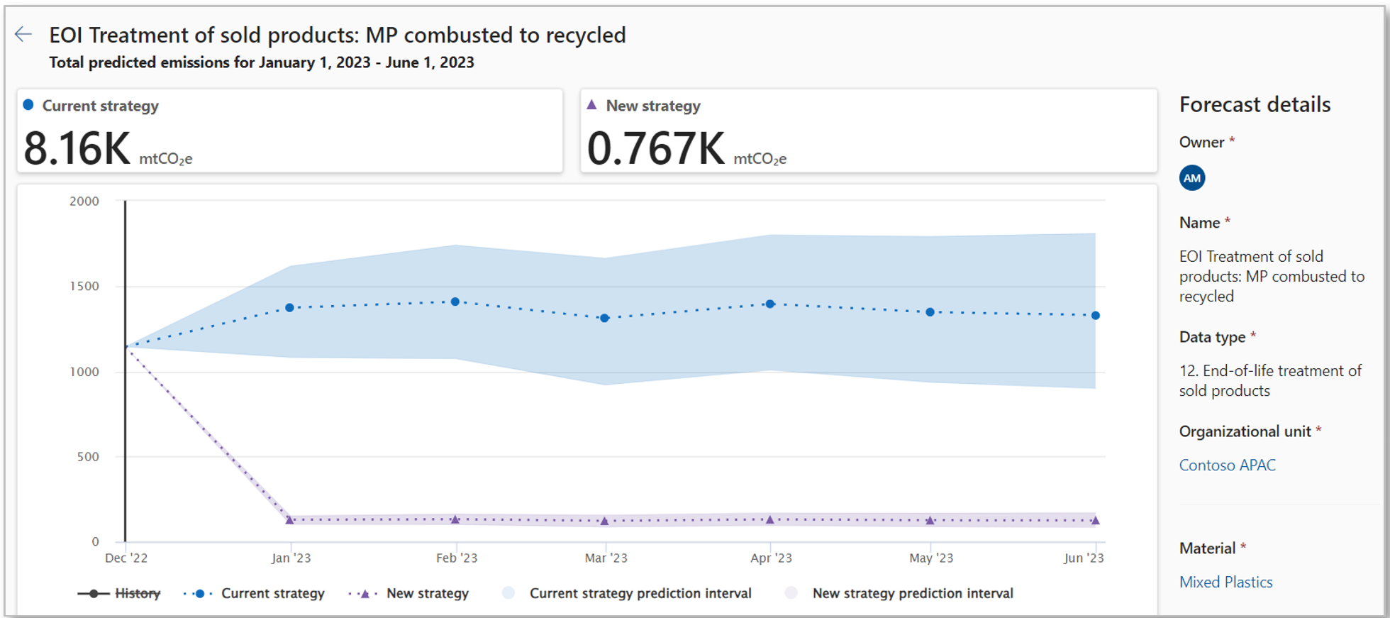
Jamie Evans, an emissions analyst at Contoso APAC, is collaborating with the team to optimize and reduce emissions associated with the end-of-life treatment of sold products in the APAC region. To achieve this optimization, Jamie plans to create a forecast that guides their decision-making process.
Of the 15 available data types, each with customizable configurations tailored to meet specific organizational needs, Jamie selects the End-of-life treatment of sold products category, which allows Jamie to assess the impact of different disposal methods on the organization’s emissions. Jamie chooses to forecast the impact of switching from combusting to recycling their mixed plastics, as that’s currently the largest contributor of emissions in this category for Contoso APAC.
To ensure that the forecasts generated are reliable, Jamie begins by examining the historical data. This examinationation provides Jamie with confidence in the accuracy of the projections. Jamie carefully notes the estimated emissions and formulates a strategy for communicating these findings back to the team.
Scenario 2: Create a layered forecast
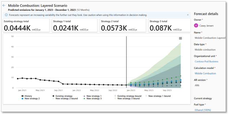
Contoso Pod Business currently operates light-duty trucks that consume Ethanol. The company aims to implement new strategies to optimize and reduce emissions from mobile combustion.
Jamie Evans, an Emissions Analyst at Contoso Pod Business, is tasked with forecasting the impact of switching from Ethanol to alternative fuel types to support decision-making.
To evaluate the effects of various mobile combustion methods, Jamie selects the Mobile Combustion category. Jamie focuses on forecasting the implications of transitioning from Ethanol to alternative fuel types, including Compressed Natural Gas (CNG), Liquefied Natural Gas (LNG), and Biodiesel.
To ensure that the forecasts generated are reliable, Jamie begins by examining the historical data. The historical data provides confidence in the accuracy of the projections. Jamie carefully notes the estimated emissions and formulates the strategies for communicating these findings back to the team.


