Esercizio - Stimare le risorse per un problema reale
L'algoritmo di fattorizzazione di Shor è uno degli algoritmi quantistici più noti. Offre un accelerazione esponenziale rispetto a qualsiasi algoritmo di factoring classico noto.
La crittografia classica usa mezzi fisici o matematici, come la difficoltà computazionale, per eseguire un'attività. Un protocollo crittografico molto diffuso è lo schema Rivest-Shamir-Adleman (RSA), che si basa sulla presunta difficoltà di fattorizzare i numeri primi usando un computer classico.
L'algoritmo di Shor implica che la crittografia a chiave pubblica possa essere decifrata con computer quantistici sufficientemente grandi. La stima delle risorse necessarie per l'algoritmo di Shor è importante per valutare la vulnerabilità di questi tipi di schemi crittografici.
Nel seguente esercizio, si calcoleranno le stime delle risorse per la fattorizzazione di un intero a 2.048 bit. Per questa applicazione, si calcoleranno le stime delle risorse fisiche direttamente dalle stime precalcolate delle risorse logiche. Per il budget degli errori tollerato, si userà $\epsilon = 1/3$.
Scrivere l'algoritmo di Shor
In Visual Studio Code, selezionare Visualizza > Riquadro comandi e selezionare Crea: Nuovo Jupyter Notebook.
Salvare il notebook come ShorRE.ipynb.
Nella prima cella, importare il pacchetto
qsharp:import qsharpUsare lo spazio
Microsoft.Quantum.ResourceEstimationdei nomi per definire una versione memorizzata nella cache dell'algoritmo di fattorizzazione integer di Shor. Aggiungere una nuova cella e copiare e incollare il codice seguente:%%qsharp open Microsoft.Quantum.Arrays; open Microsoft.Quantum.Canon; open Microsoft.Quantum.Convert; open Microsoft.Quantum.Diagnostics; open Microsoft.Quantum.Intrinsic; open Microsoft.Quantum.Math; open Microsoft.Quantum.Measurement; open Microsoft.Quantum.Unstable.Arithmetic; open Microsoft.Quantum.ResourceEstimation; operation RunProgram() : Unit { let bitsize = 31; // When choosing parameters for `EstimateFrequency`, make sure that // generator and modules are not co-prime let _ = EstimateFrequency(11, 2^bitsize - 1, bitsize); } // In this sample we concentrate on costing the `EstimateFrequency` // operation, which is the core quantum operation in Shors algorithm, and // we omit the classical pre- and post-processing. /// # Summary /// Estimates the frequency of a generator /// in the residue ring Z mod `modulus`. /// /// # Input /// ## generator /// The unsigned integer multiplicative order (period) /// of which is being estimated. Must be co-prime to `modulus`. /// ## modulus /// The modulus which defines the residue ring Z mod `modulus` /// in which the multiplicative order of `generator` is being estimated. /// ## bitsize /// Number of bits needed to represent the modulus. /// /// # Output /// The numerator k of dyadic fraction k/2^bitsPrecision /// approximating s/r. operation EstimateFrequency( generator : Int, modulus : Int, bitsize : Int ) : Int { mutable frequencyEstimate = 0; let bitsPrecision = 2 * bitsize + 1; // Allocate qubits for the superposition of eigenstates of // the oracle that is used in period finding. use eigenstateRegister = Qubit[bitsize]; // Initialize eigenstateRegister to 1, which is a superposition of // the eigenstates we are estimating the phases of. // We first interpret the register as encoding an unsigned integer // in little endian encoding. ApplyXorInPlace(1, eigenstateRegister); let oracle = ApplyOrderFindingOracle(generator, modulus, _, _); // Use phase estimation with a semiclassical Fourier transform to // estimate the frequency. use c = Qubit(); for idx in bitsPrecision - 1..-1..0 { within { H(c); } apply { // `BeginEstimateCaching` and `EndEstimateCaching` are the operations // exposed by Azure Quantum Resource Estimator. These will instruct // resource counting such that the if-block will be executed // only once, its resources will be cached, and appended in // every other iteration. if BeginEstimateCaching("ControlledOracle", SingleVariant()) { Controlled oracle([c], (1 <<< idx, eigenstateRegister)); EndEstimateCaching(); } R1Frac(frequencyEstimate, bitsPrecision - 1 - idx, c); } if MResetZ(c) == One { set frequencyEstimate += 1 <<< (bitsPrecision - 1 - idx); } } // Return all the qubits used for oracles eigenstate back to 0 state // using Microsoft.Quantum.Intrinsic.ResetAll. ResetAll(eigenstateRegister); return frequencyEstimate; } /// # Summary /// Interprets `target` as encoding unsigned little-endian integer k /// and performs transformation |k⟩ ↦ |gᵖ⋅k mod N ⟩ where /// p is `power`, g is `generator` and N is `modulus`. /// /// # Input /// ## generator /// The unsigned integer multiplicative order ( period ) /// of which is being estimated. Must be co-prime to `modulus`. /// ## modulus /// The modulus which defines the residue ring Z mod `modulus` /// in which the multiplicative order of `generator` is being estimated. /// ## power /// Power of `generator` by which `target` is multiplied. /// ## target /// Register interpreted as LittleEndian which is multiplied by /// given power of the generator. The multiplication is performed modulo /// `modulus`. internal operation ApplyOrderFindingOracle( generator : Int, modulus : Int, power : Int, target : Qubit[] ) : Unit is Adj + Ctl { // The oracle we use for order finding implements |x⟩ ↦ |x⋅a mod N⟩. We // also use `ExpModI` to compute a by which x must be multiplied. Also // note that we interpret target as unsigned integer in little-endian // encoding by using the `LittleEndian` type. ModularMultiplyByConstant(modulus, ExpModI(generator, power, modulus), target); } /// # Summary /// Performs modular in-place multiplication by a classical constant. /// /// # Description /// Given the classical constants `c` and `modulus`, and an input /// quantum register (as LittleEndian) |𝑦⟩, this operation /// computes `(c*x) % modulus` into |𝑦⟩. /// /// # Input /// ## modulus /// Modulus to use for modular multiplication /// ## c /// Constant by which to multiply |𝑦⟩ /// ## y /// Quantum register of target internal operation ModularMultiplyByConstant(modulus : Int, c : Int, y : Qubit[]) : Unit is Adj + Ctl { use qs = Qubit[Length(y)]; for (idx, yq) in Enumerated(y) { let shiftedC = (c <<< idx) % modulus; Controlled ModularAddConstant([yq], (modulus, shiftedC, qs)); } ApplyToEachCA(SWAP, Zipped(y, qs)); let invC = InverseModI(c, modulus); for (idx, yq) in Enumerated(y) { let shiftedC = (invC <<< idx) % modulus; Controlled ModularAddConstant([yq], (modulus, modulus - shiftedC, qs)); } } /// # Summary /// Performs modular in-place addition of a classical constant into a /// quantum register. /// /// # Description /// Given the classical constants `c` and `modulus`, and an input /// quantum register (as LittleEndian) |𝑦⟩, this operation /// computes `(x+c) % modulus` into |𝑦⟩. /// /// # Input /// ## modulus /// Modulus to use for modular addition /// ## c /// Constant to add to |𝑦⟩ /// ## y /// Quantum register of target internal operation ModularAddConstant(modulus : Int, c : Int, y : Qubit[]) : Unit is Adj + Ctl { body (...) { Controlled ModularAddConstant([], (modulus, c, y)); } controlled (ctrls, ...) { // We apply a custom strategy to control this operation instead of // letting the compiler create the controlled variant for us in which // the `Controlled` functor would be distributed over each operation // in the body. // // Here we can use some scratch memory to save ensure that at most one // control qubit is used for costly operations such as `AddConstant` // and `CompareGreaterThenOrEqualConstant`. if Length(ctrls) >= 2 { use control = Qubit(); within { Controlled X(ctrls, control); } apply { Controlled ModularAddConstant([control], (modulus, c, y)); } } else { use carry = Qubit(); Controlled AddConstant(ctrls, (c, y + [carry])); Controlled Adjoint AddConstant(ctrls, (modulus, y + [carry])); Controlled AddConstant([carry], (modulus, y)); Controlled CompareGreaterThanOrEqualConstant(ctrls, (c, y, carry)); } } } /// # Summary /// Performs in-place addition of a constant into a quantum register. /// /// # Description /// Given a non-empty quantum register |𝑦⟩ of length 𝑛+1 and a positive /// constant 𝑐 < 2ⁿ, computes |𝑦 + c⟩ into |𝑦⟩. /// /// # Input /// ## c /// Constant number to add to |𝑦⟩. /// ## y /// Quantum register of second summand and target; must not be empty. internal operation AddConstant(c : Int, y : Qubit[]) : Unit is Adj + Ctl { // We are using this version instead of the library version that is based // on Fourier angles to show an advantage of sparse simulation in this sample. let n = Length(y); Fact(n > 0, "Bit width must be at least 1"); Fact(c >= 0, "constant must not be negative"); Fact(c < 2 ^ n, $"constant must be smaller than {2L ^ n}"); if c != 0 { // If c has j trailing zeroes than the j least significant bits // of y will not be affected by the addition and can therefore be // ignored by applying the addition only to the other qubits and // shifting c accordingly. let j = NTrailingZeroes(c); use x = Qubit[n - j]; within { ApplyXorInPlace(c >>> j, x); } apply { IncByLE(x, y[j...]); } } } /// # Summary /// Performs greater-than-or-equals comparison to a constant. /// /// # Description /// Toggles output qubit `target` if and only if input register `x` /// is greater than or equal to `c`. /// /// # Input /// ## c /// Constant value for comparison. /// ## x /// Quantum register to compare against. /// ## target /// Target qubit for comparison result. /// /// # Reference /// This construction is described in [Lemma 3, arXiv:2201.10200] internal operation CompareGreaterThanOrEqualConstant(c : Int, x : Qubit[], target : Qubit) : Unit is Adj+Ctl { let bitWidth = Length(x); if c == 0 { X(target); } elif c >= 2 ^ bitWidth { // do nothing } elif c == 2 ^ (bitWidth - 1) { ApplyLowTCNOT(Tail(x), target); } else { // normalize constant let l = NTrailingZeroes(c); let cNormalized = c >>> l; let xNormalized = x[l...]; let bitWidthNormalized = Length(xNormalized); let gates = Rest(IntAsBoolArray(cNormalized, bitWidthNormalized)); use qs = Qubit[bitWidthNormalized - 1]; let cs1 = [Head(xNormalized)] + Most(qs); let cs2 = Rest(xNormalized); within { for i in IndexRange(gates) { (gates[i] ? ApplyAnd | ApplyOr)(cs1[i], cs2[i], qs[i]); } } apply { ApplyLowTCNOT(Tail(qs), target); } } } /// # Summary /// Internal operation used in the implementation of GreaterThanOrEqualConstant. internal operation ApplyOr(control1 : Qubit, control2 : Qubit, target : Qubit) : Unit is Adj { within { ApplyToEachA(X, [control1, control2]); } apply { ApplyAnd(control1, control2, target); X(target); } } internal operation ApplyAnd(control1 : Qubit, control2 : Qubit, target : Qubit) : Unit is Adj { body (...) { CCNOT(control1, control2, target); } adjoint (...) { H(target); if (M(target) == One) { X(target); CZ(control1, control2); } } } /// # Summary /// Returns the number of trailing zeroes of a number /// /// ## Example /// ```qsharp /// let zeroes = NTrailingZeroes(21); // = NTrailingZeroes(0b1101) = 0 /// let zeroes = NTrailingZeroes(20); // = NTrailingZeroes(0b1100) = 2 /// ``` internal function NTrailingZeroes(number : Int) : Int { mutable nZeroes = 0; mutable copy = number; while (copy % 2 == 0) { set nZeroes += 1; set copy /= 2; } return nZeroes; } /// # Summary /// An implementation for `CNOT` that when controlled using a single control uses /// a helper qubit and uses `ApplyAnd` to reduce the T-count to 4 instead of 7. internal operation ApplyLowTCNOT(a : Qubit, b : Qubit) : Unit is Adj+Ctl { body (...) { CNOT(a, b); } adjoint self; controlled (ctls, ...) { // In this application this operation is used in a way that // it is controlled by at most one qubit. Fact(Length(ctls) <= 1, "At most one control line allowed"); if IsEmpty(ctls) { CNOT(a, b); } else { use q = Qubit(); within { ApplyAnd(Head(ctls), a, q); } apply { CNOT(q, b); } } } controlled adjoint self; }
Stimare l'algoritmo di Shor
Stimare ora le risorse fisiche per l'operazione RunProgram usando le ipotesi predefinite. Aggiungere una nuova cella e copiare e incollare il codice seguente:
result = qsharp.estimate("RunProgram()")
result
La funzione qsharp.estimate crea un oggetto risultato, che può essere usato per visualizzare una tabella con il conteggio complessivo delle risorse fisiche. È possibile controllare i dettagli dei costi comprimendo i gruppi, che includono altre informazioni.
Ad esempio, comprimere il gruppo di Parametri qubit logici per vedere che la distanza del codice è 21 e il numero di qubit fisici è 882.
| Parametro qubit logico | Valore |
|---|---|
| Schema Correzione degli errori quantistici | surface_code |
| Distanza di codice | 21 |
| Qubit fisici | 882 |
| Tempo ciclo logico | 8 millisec |
| Frequenza di errore del qubit logico | 3.00E-13 |
| Attraversamento del prefactoring | 0.03 |
| Soglia di correzione degli errori | 0,01 |
| Formula tempo del ciclo logico | (4 * twoQubitGateTime + 2 * oneQubitMeasurementTime) * codeDistance |
| Formula qubit fisici | 2 * codeDistance * codeDistance |
Suggerimento
Per una versione più compatta della tabella di output, è possibile usare result.summary.
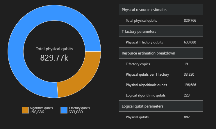
Diagramma spaziale
La distribuzione dei qubit fisici usati per l'algoritmo e le factory T è un fattore che potrebbe influire sulla progettazione dell'algoritmo. È possibile usare il pacchetto qsharp-widgets per visualizzare questa distribuzione per comprendere meglio i requisiti di spazio stimati dell'algoritmo.
from qsharp_widgets import SpaceChart
SpaceChart(result)
In questo esempio, il numero di qubit fisici necessari per eseguire l'algoritmo è 829766, di cui 196686 sono qubit di algoritmo e 633080 sono qubit di T factory.
Confrontare le stime delle risorse per tecnologie qubit diverse
Lo strumento di stima delle risorse di Azure Quantum consente di eseguire più configurazioni dei parametri di destinazione e confrontare i risultati. Ciò è utile quando si vuole confrontare il costo di modelli qubit diversi, schemi QEC o budget di errore.
È anche possibile creare un elenco di parametri di stima usando l'oggetto EstimatorParams.
from qsharp.estimator import EstimatorParams, QubitParams, QECScheme, LogicalCounts

labels = ["Gate-based µs, 10⁻³", "Gate-based µs, 10⁻⁴", "Gate-based ns, 10⁻³", "Gate-based ns, 10⁻⁴", "Majorana ns, 10⁻⁴", "Majorana ns, 10⁻⁶"]

params = EstimatorParams(6)
params.error_budget = 0.333
params.items[0].qubit_params.name = QubitParams.GATE_US_E3
params.items[1].qubit_params.name = QubitParams.GATE_US_E4
params.items[2].qubit_params.name = QubitParams.GATE_NS_E3
params.items[3].qubit_params.name = QubitParams.GATE_NS_E4
params.items[4].qubit_params.name = QubitParams.MAJ_NS_E4
params.items[4].qec_scheme.name = QECScheme.FLOQUET_CODE
params.items[5].qubit_params.name = QubitParams.MAJ_NS_E6
params.items[5].qec_scheme.name = QECScheme.FLOQUET_CODE

qsharp.estimate("RunProgram()", params=params).summary_data_frame(labels=labels)
| Modello Qubit | Qubit logici | Profondità logica | T states | Distanza di codice | T factory | Frazione T factory | Qubit fisici | rQOPS | Runtime fisico |
|---|---|---|---|---|---|---|---|---|---|
| Basato su gate µs 10⁻³ | 223 3,64M | 4.70M | 17 | 13 | 40.54 % | 216.77k | 21,86 k | 10 ore | |
| Basato su gate µs 10⁻⁴ | 223 | 3,64 M | 4.70M | 9 | 14 | 43.17 % | 63,57 k | 41.30k | 5 ore |
| Basato su gate ns 10⁻³ | 223 3,64M | 4.70M | 17 | 16 | 69.08 % | 416.89k | 32,79M | 25 sec | |
| Basato su gate ns 10⁻⁴ | 223 3,64M | 4.70M | 9 | 14 | 43.17 % | 63,57 k | 61,94M | 13 sec | |
| Majorana ns 10⁻⁴ | 223 3,64M | 4.70M | 9 | 19 | 82.75 % | 501.48k | 82.59M | 10 sec | |
| Majorana ns 10⁻⁶ | 223 3,64M | 4.70M | 5 | 13 | 31.47 % | 42.96k | 148.67M | 5 sec |
Estrarre stime delle risorse dai conteggi delle risorse logiche
Se si dispone già di alcune stime per un'operazione, lo strumento di stima delle risorse permette di integrare queste stime nel costo totale del programma, al fine di ridurre il tempo di esecuzione. È possibile usare la classe LogicalCounts per estrarre le stime logiche delle risorse dai valori di stima delle risorse precalcolati.
Selezionare Codice per aggiungere una nuova cella e quindi immettere ed eseguire il codice seguente:
logical_counts = LogicalCounts({
    'numQubits': 12581,
    'tCount': 12,
    'rotationCount': 12,
    'rotationDepth': 12,
    'cczCount': 3731607428,
    'measurementCount': 1078154040})

logical_counts.estimate(params).summary_data_frame(labels=labels)
| Modello Qubit | Qubit logici | Profondità logica | T states | Distanza di codice | T factory | Frazione T factory | Qubit fisici | Runtime fisico |
|---|---|---|---|---|---|---|---|---|
| Basato su gate µs 10⁻³ | 25481 | 1,2e+10 | 1,5e+10 | 27 | 13 | 0,6% | 37,38M | 6 anni |
| Basato su gate µs 10⁻⁴ | 25481 | 1,2e+10 | 1,5e+10 | 13 | 14 | 0,8% | 8,68M | 3 anni |
| Basato su gate ns 10⁻³ | 25481 | 1,2e+10 | 1,5e+10 | 27 | 15 | 1,3% | 37,65M | 2 giorni |
| Basato su gate ns 10⁻⁴ | 25481 | 1,2e+10 | 1,5e+10 | 13 | 18 | 1,2% | 8,72M | 18 ore |
| Majorana ns 10⁻⁴ | 25481 | 1,2e+10 | 1,5e+10 | 15 | 15 | 1,3% | 26,11M | 15 ore |
| Majorana ns 10⁻⁶ | 25481 | 1,2e+10 | 1,5e+10 | 7 | 13 | 0,5% | 6,25M | 7 ore |
Conclusione
Nel peggiore dei casi, un computer quantico che usa qubit µs basati su gate (qubit che hanno tempi di funzionamento nel regime dei nanosecondi, come i qubit superconduttori) e un codice QEC di superficie, avrebbe bisogno di sei anni e 37,38 milioni di qubit per fattorizzare un intero a 2.048 bit usando l'algoritmo di Shor.
Se viene usata una tecnologia di qubit diversa, ad esempio qubit a ioni ns basati su gate e lo stesso codice di superficie, il numero di qubit non cambia molto, ma il tempo di esecuzione diventa di due giorni nel caso peggiore dei casi e di 18 ore nell'ipotesi più ottimistica. Se si cambia la tecnologia dei qubit e il codice QEC, ad esempio usando qubit basati su Majorana, la fattorizzazione di un intero a 2.048 bit usando l'algoritmo di Shor potrebbe essere eseguita in ore con un array di 6,25 milioni di qubit nel migliore dei casi.
Dall'esperimento, è possibile concludere che l'uso di qubit di Majorana e di un codice QEC Floquet è la scelta migliore per eseguire l'algoritmo di Shor e fattorizzare un integer a 2.048 bit.