Build a recommendation system with the support for graph data in SQL Server 2017 and Azure SQL DB
Authored by Arvind Shyamsundar and Shreya Verma
Reviewed by Dimitri Furman, Joe Sack, Sanjay Mishra, Denzil Ribeiro, Mike Weiner, Rajesh Setlem
Graphs are a very common way to represent networks and relationships between objects. Historically, it is not easy to represent such data structures in relational databases like SQL Server and Azure SQL DB. To address this requirement, in November 2016 (through a private preview program for a set of early adopter customers) we introduced extensions to which allow us to natively store and query graphs inside the database on Azure SQL DB.
We recently made these features publicly available as part of the SQL Server 2017 CTP 2.0 release (note that the feature is still in private preview for Azure SQL DB at this time). Please review this related blog post for an overview of the feature. In our blog post we look at a typical use case for graph data in SQL Server and Azure SQL DB.
Scenario
A common scenario we've seen with our early adopter customers is their interest to use graph technology to implement 'recommendation systems'. For this walkthrough, imagine we have to implement a recommendation system for songs. Specifically, let's imagine a scenario where there's a user who likes Lady Gaga's song 'Just Dance'. Now, our objective is to implement a recommendation system which will suggest songs which are similar to 'Just Dance'. So, how do we get started? First, we need data!
What data can we use?
Many approaches to implementing recommendation systems involve using two distinct sets of data: one which contains users, and the other which contains details of the entities that those users are related to.
- In retail scenarios, these would be the products purchased by the user.
- In our current scenario, these are the songs which those users listened to.
It so happens that there is an amazing source of such data for songs and ‘user tastes’ (which songs did each user listen to) available online. This dataset is called the Million Song Dataset (MSD), and while it has a lot of other information, the specific subset of data that is of immediate interest to us is summarized below:
- The list of all the songs is contained in a delimited file available here. There are a million songs in this dataset.
- On the MSD website there is a link to another dataset called the ‘User Taste Profile’ data which contains (anonymized) user listening profiles and that is available here. There are a million unique users, and a total of 48 million ‘relationships’ (each corresponding to a row in this file) in this dataset.
What algorithm?
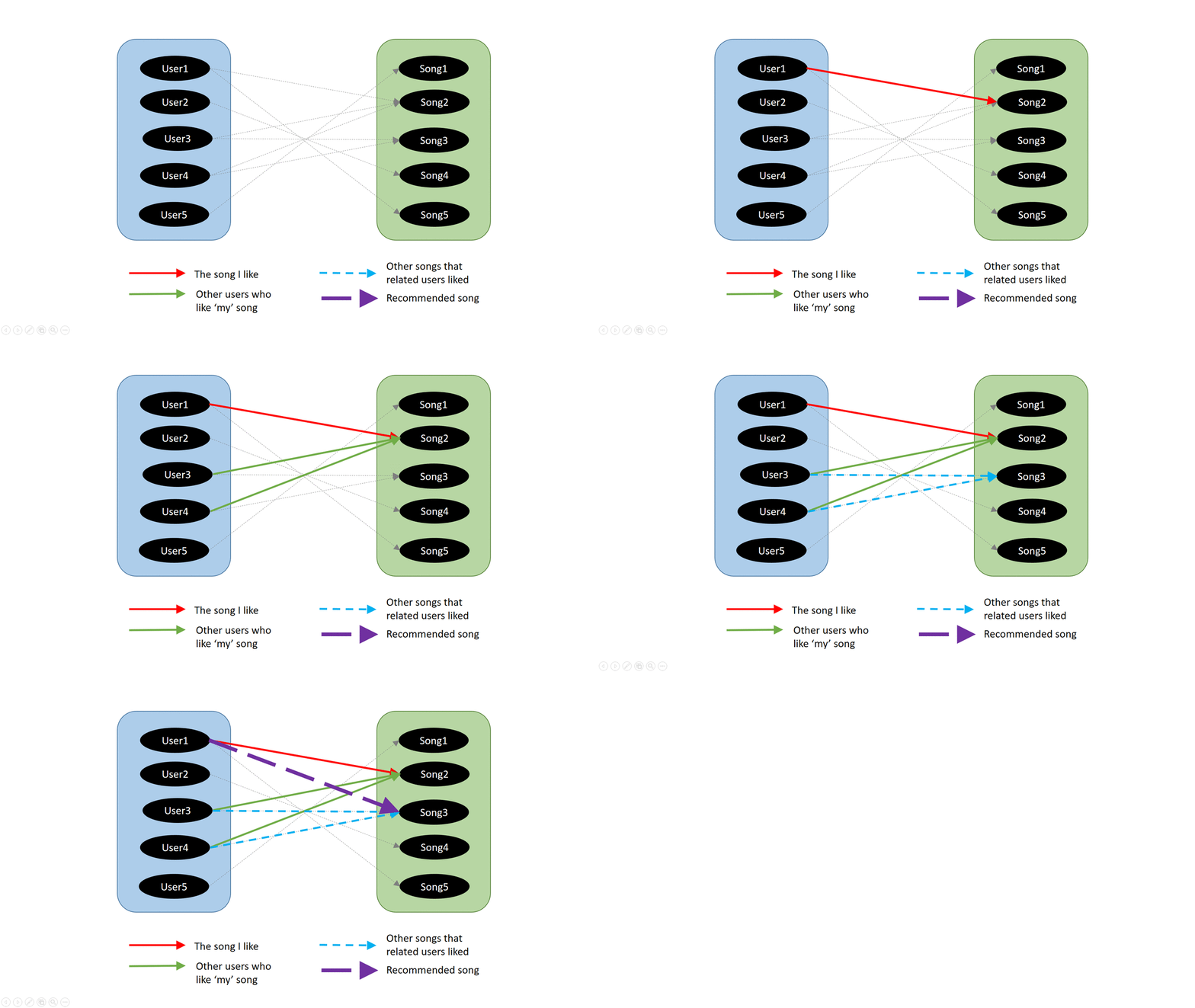
Now that we know what data is available to us, let’s think about the algorithm to be used. A standard approach called collaborative filtering can be used in conjunction with our graph data. Presented below is a simplified graphical representation of the algorithm that we will use.
As you can see from the animation, the algorithm is quite simple:
- First, we identify the user and ‘current’ song to start with (red line)
- Next, we identify the other users who have also listened to this song (green line)
- Then we find the other songs which those other users have also listened to (blue, dotted line)
- Finally, we direct the current user to the top songs from those other songs, prioritized by the number of times they were listened to (this is represented by the thick violet line.)
The algorithm above is quite simple, but as you will see it is quite effective in meeting our requirement. Now, let’s see how to actually implement this in SQL Server 2017.
Implementation
To begin, we recommend that you quickly review this feature overview video as well as the official documentation links for more details on the new functionality:
- An overview of Graph data in SQL Server
- Architecture details for Graph data in SQL Server
- The official sample for Graph data in SQL Server
Once you have the background, it’s easy to understand how to represent the scenario as ‘graph tables’ in SQL Server 2017. We will create two ‘node’ tables – one for the users and one for the songs. We will then ‘connect’ these two node tables with an ‘edge’ table. Here’s a quick visual summary of what we will be doing:
Importing the data
Now, let’s get to the nuts and bolts! The first step is to declare tables into which we will insert the source data. These ‘staging’ tables are ‘regular’ tables and have no ‘graph’ attributes. Here are the scripts for this:
The next step is to use the OPENROWSET BULK functionality to rapidly ingest the text files into their staging tables in SQL Server. Here are the scripts for this:
Constructing the graph
Once we have the raw data in staging tables, we can then 'convert' them into their Graph equivalents. Here are the table definitions; note the usage of AS NODE and AS EDGE to define the tables involved in the graph:
To actually ‘convert’ the data, we use INSERT...SELECT statements as shown below:
Querying the graph
Now that we have all the data in the 'graph' form, we can proceed to use the new MATCH function to express our query over the set of nodes and edges. The query below finds songs that are similar to Lady Gaga's song called 'Just Dance'!
Optimizing performance
The above query performs relatively quickly (in around 3 seconds on a laptop with an i7 processor). Consider that this query has to deal with a million users, a million songs and 48 million relationships between those entities. Most of the cost is taken by the time to scan through the tables, one row at a time and then match them using hash joins, as you can visualize by looking at the execution plan:
While 3 seconds is not bad, can we make this even faster? The good news is that in SQL Server 2017 CTP 2.0, graph tables support clustered columnstore indexes. While the compression offered is definitely going to help reduce I/O, the bigger benefit is that queries on these tables leverage the ‘batch-mode’ execution which allows much faster execution of queries. This is really useful for us given that the above query is doing large aggregations (GROUP BY). Let's proceed to create these clustered columnstore indexes:
Once we create these indexes, the performance actually improves substantially and reduces the query execution time to half a second, which is 6x faster than before. That's really impressive considering the sheer amount of data that the query needs to look at to arrive at the result!
Let’s take a minute to look at the new execution plan. Observe the ‘Batch mode’ execution highlighted below:
The other interesting thing to note is the new adaptive join type highlighted above. This is great to see - queries on graph data benefit with these new query processing improvements inside SQL Server 2107!
Let’s summarize the ‘before’ and ‘after’ states:
Query execution time (seconds) |
Logical Reads (for the Likes table) |
Space occupied by the Likes table on disk |
|
Heap tables |
3.6 |
588388 |
3.4GB |
Clustered columstore |
0.6 |
174852 |
1.7GB |
In summary, having graph data inside SQL Server allows database administrators and developers to leverage the familiar, mature and robust query processing capabilities within SQL Server. This is crucial to reducing the learning curve and likely complexity associated with using other technologies to store and query graph data.
Visualizing graphs
While we can use external applications and tools like PowerBI to visualize graphs, the ‘icing on the cake’ is the fact that we can use R Services in SQL Server to visualize graph data. With an open-source R package called 'igraph' we can visualize graphs relatively easily and render them to standard image formats like PNG. Here is a code snippet showing you how that can be done:
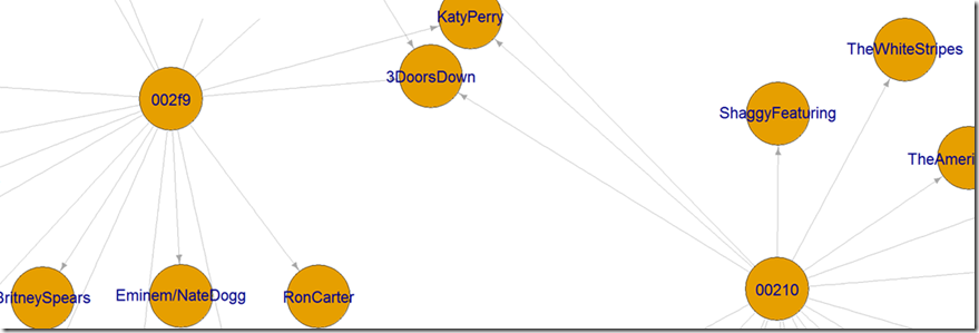
Here's a section of the visualization (refer the comments in the above script to understand what the visualization represents) generated. While it is quite basic, but as you can see it is functionally very useful:
Conclusion
The support for graph data in SQL Server 2017 is an exciting new development and opens up doors to a new category of workloads which can leverage this functionality. It is one more step in bringing algorithms and intelligence closer to where the data resides.
Recommendation systems (such as the simple example presented here), fraud detection systems, content and asset management and many other scenarios can also benefit from the integration that graph data in SQL Server 2017 offers. The support for graph data in the database will be also be publicly available for Azure SQL DB in due course of time.
The complete code for this walkthrough is available here. Please use the Comments section below to ask questions and provide your feedback. We are eager to hear from you!
Citations
Thierry Bertin-Mahieux, Daniel P.W. Ellis, Brian Whitman, and Paul Lamere. The Million Song Dataset. In Proceedings of the 12th International Society for Music Information Retrieval Conference (ISMIR 2011), 2011.
The Echo Nest Taste profile subset, the official user data collection for the Million Song Dataset, available at: https://labrosa.ee.columbia.edu/millionsong/tasteprofile
Comments
- Anonymous
May 02, 2017
The comment has been removed- Anonymous
May 17, 2017
This was sorted out offline with Aditya - he needed to use the RAW view in GitHub to get the correct files.
- Anonymous
- Anonymous
July 22, 2017
The comment has been removed- Anonymous
July 24, 2017
@pcofre: There was a bug with the echonesttracks.xml format file. I've fixed it now. Can you please pull the latest version and check again?- Anonymous
July 25, 2017
Thanks ArvindNow it works! Thanks!
- Anonymous
- Anonymous
- Anonymous
July 30, 2017
For the visualization part, when defining the filename, I had to change the double quotation by two single quotes surrounding the path c:\MSD\plot1.png to make it work!old: png(filename = "c:\MSD\plot1.png", ...new: png(filename = ''c:\MSD\plot1.png'', ...


