Feature Engineering using R
Feature Engineering is paramount in building a good predictive model. It's significant to obtain a deep understanding of the data that is being used for analysis. The characteristics of the selected features are definitive of a good training model.
Why is Feature Engineering important?
- Too many features or redundant features could increase the run time complexity of training the model. In some cases, it could lead to Over Fitting as the model might attempt to fit the data too perfectly.
- Understanding and visualizing the data and how certain features are more important than the others helps in reducing overall noise and improving the accuracy of the system.
- Defying the Curse of Dimensionality - ensuring not to increase the number of features above the threshold that would only degrade model performance.
- Not all features are numeric, so some kind of transformation is required. (e.g. creating the feature vector from textual data)
This blog aims to go through a few well-known methods for selecting, filtering or constructing new features in a quick R way as opposed to helping you understand the theoretical mathematics or statistics behind it. Note that this is by no means an exhaustive list of methods and I try to keep the concepts crisp and to the point.
How to categorize Feature Engineering? Here I approach them as the follows:
- Feature Filters: selecting a subset of relevant features from the feature set.
- Wrapper Method: evaluates different feature space based on some criteria to pick the best possible subset.
- Feature Extraction and Construction: extracting and creating new features from existing features.
- Embedded Methods: feature selection that is performed as a part of the training process.
For most of the examples, the default data set in R is used. To quickly list all the data sets available to you from R:
> data()
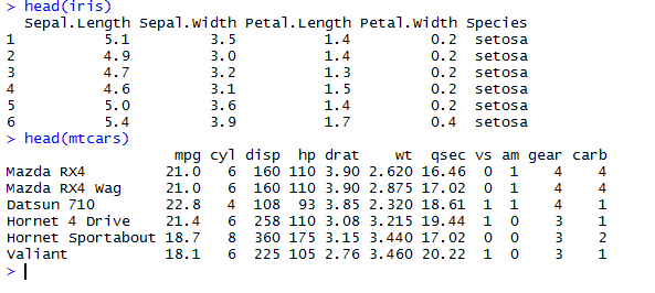
We will either use mtcars or iris data sets for most of the examples. As most of these data sets are very small, some of the below examples could exhibit over-fitting, fixing it is not in the scope of this blog.
Feature set of iris and mtcars:
Feature Filters
Filter methods are used to select a subset of the existing features based on certain criteria. Features chosen by filters are generic to the feature variables and are not tuned to any specific machine learning algorithm that is used. Filter methods can be used to pre-process the data to select meaningful features and reduce the feature space and avoid over-fitting, especially when there is a small number of data points when compared to the number of features.
Correlation coefficients
Correlation coefficient is a score that helps to understand the dependence and relationship between two variables, say X and Y. It's helps filtering features that could be duplicates - if it has a strong correlation to other features and also picking features that are correlated to the response variable.
Most commonly used method is Pearson's Correlation Coefficient that is used to score linear dependence between two variables. The mtcars contains data about 32 cars including features like miles/gallon, weight, gross horsepower, etc. Let's use Pearson's method to understand the relationship between mpg and car weight.
Visualize the two parameters:
plot(mtcars$wt, mtcars$mpg, col="red", xlab = "Weight of the cars", ylab = "Miles per gallon", pch=16, main = "Pearson Correlation")
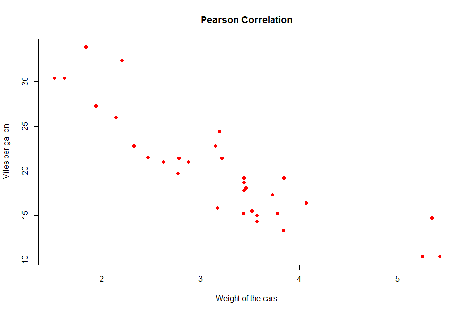
Notice the pattern as the weight of the car increases. To find the correlation value, use RxCor()
 > form <- ~ wt + mpg + cyl
> rxCor(form, data = mtcars)
Rows Read: 32, Total Rows Processed: 32, Total Chunk Time: 0.001 seconds
Computation time: 0.004 seconds.
 wt mpg cyl
wt 1.0000000 -0.8676594 0.7824958
mpg  -0.8676594 1.0000000 -0.8521620
cyl 0.7824958 -0.8521620 1.0000000
Correlation Coefficients are usually between -1 and +1 representing strong negative and strong positive correlation respectively. If the value is 0, then there is no correlation between the two variables. Collinearity happens when two variables are highly correlated with each other. Though this would not degrade predictive power of your model it makes it harder to evaluate the importance of individual predictors.
Perfectly correlated variables are redundant and might not add value to the model (and if removed, would be quicker to train). However, two variables that are not strongly correlated could still be of importance to the model. When in doubt, it's safer to train the model and observe it's performance.
To obtain more information about the correlation, R has a cor.test() method:
 >cor.test(x = mtcars$wt, y = mtcars$mpg)
 Pearson's product-moment correlation
 data: mtcars$wt and mtcars$mpg
 t = -9.559, df = 30, p-value = 1.294e-10
 alternative hypothesis: true correlation is not equal to 0
 95 percent confidence interval:
 -0.9338264 -0.7440872
 sample estimates:
 cor
 -0.8676594
(use method="spearman" or "kendall" in cor() to understand monotonic relationships).
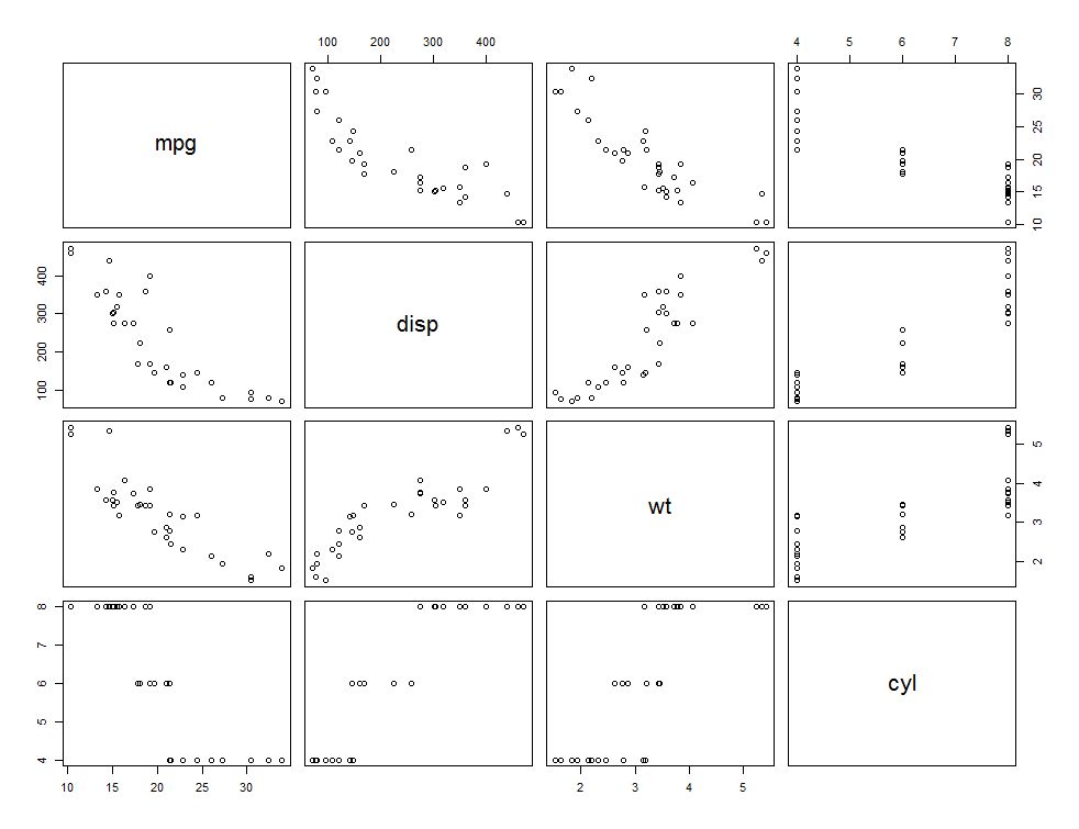
You could also plot(mtcars) or cor(mtcars) to obtain the value and plot for all the possible correlations. To simplify just a subset of the features, you could use:
pairs(~mpg + disp + wt + cyl, data=mtcars, main=”Scatterplot Matrix”)
Mutual Information
Mutual Information of the predictors and the response variable (or the class) calculates how important the inclusion or exclusion of that particular feature is in predicting the correct class. It estimates the 'amount of information' that is shared between two random variables say X and Y. So knowing X, would reduce the uncertainty of Y. It helps determine which feature among a given feature vector is most useful in determining the response variable.
MI uses the probability distribution of the variables unlike Correlation and is not limited to understanding linear dependencies. After gathering the mutual importance of a feature, eliminating non informative features and retaining the important features could potentially reduce noise and help accuracy.
If for the iris dataset, we are predicting the Species - we can use information.gain() function in R that calculates the MI between the features and the response variable.
 > library(FSelector)
> ig_values <- information.gain(Species~., iris)
> ig_values
 attr_importance
Sepal.Length 0.4521286
Sepal.Width 0.2672750
Petal.Length 0.9402853
Petal.Width 0.9554360

> # filter the top K features and use it to create the model formula
> top_k_features <- cutoff.k(ig_values, 2)
> f <- as.simple.formula(top_k_features, "Species")
> f
Species ~ Petal.Width + Petal.Length
Microsoft R Server has a quick way to use Mutual Information as a part of Feature Selection while training a model. In this example, for training a logistic regression model, specify the top N features that should be picked based on Mutual Information:
 logistic_Mod <- rxLogisticRegression(Species ~ Petal.Width + Petal.Length + Sepal.Width + Sepal.Length, data = iris, l1Weight = 0,
type = "multi", mlTransforms = list(selectFeatures(Species ~ Petal.Width + Petal.Length + Sepal.Width + Sepal.Length, mode = mutualInformation(numFeaturesToKeep = 2))))
Wrapper Method:
Another common attempt to perform Feature Selection is by using Wrapper Methods.
When thinking of which features could matter to our model, an intuitive approach that might have crossed your mind is observing the model's accuracy for all combination of features. This 'brute-force' method, depending on the size of the data set might demand enormous computation time and space.
Greedy search strategies could be devised to solve this problem. This is a extensively researched subject but for the limited scope of the blog we will keep it succinct.
An easy approach would be to evaluate the feature individually and select top N features that score good accuracy.
However, testing the model repeatedly with only one of the features at a time, we will miss out on the information that would be obtained from the feature dependencies. So this might be naïve.
Forward Selection:
This is a simple greedy algorithm where you start with a feature set of just one feature and sequentially add the next best feature (from highest performing feature in the previous approach) and update the model continuing to observe the model performance. This method would be tedious when your feature space is large and it does not account for features that were already added to the feature set that are probably degrading the performance of the model.
Backward Selection:
Backward Selection is the reverse approach of the Forward Selection, wherein we start with all the features and then iteratively remove the least performing feature while updating the model. This would help understand if the least ranked feature was indeed useful.
Caret package in R has a function called Recursive Feature Elimination (rfe) that does this.
We will go back to using mtcars for this example and predict the mpg given the rest of the features.
 > library(caret)
> rfe_controller <- rfeControl(functions=lmFuncs, method="repeatedcv", repeats = 5, verbose = FALSE)
> size <- c(1:10)
> lm_Profiler <- rfe(mtcars[,2:11], mtcars[,1], sizes = subsets, rfeControl = rfe_controller)
> lm_Profiler
Recursive feature selection
Outer resampling method: Cross-Validated (10 fold, repeated 5 times)
Resampling performance over subset size:
Variables RMSE Rsquared RMSESD RsquaredSD Selected
 1 3.344 0.7890 1.3635 0.24535
 2 2.823 0.8675 1.0021 0.17448
 3 2.388 0.9241 0.8036 0.08555
 4 2.226 0.9380 0.7667 0.06445 *
 5 2.375 0.9281 0.8180 0.07419
 6 2.308 0.9347 0.7448 0.06735
 7 2.336 0.9331 0.8305 0.07397
 8 2.359 0.9285 0.8605 0.07120
 9 2.300 0.9331 0.8469 0.07528
 10 2.285 0.9338 0.8522 0.07145
The top 4 variables (out of 4):
 disp, wt, hp, cyl
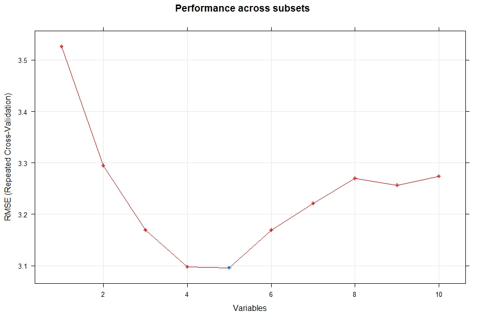
plot(lm_Profiler)
Plot the lm_Profiler to visualize the performance across different subsets.
Feature Extraction or Construction:
Sometimes based on the domain knowledge you have about the data, it might be helpful to manually construct features from existing features. This could be - aggregating a set of features into one column, splitting a feature into multiple features, using frequency of certain columns as a feature, deconstructing dates to represent number of days from a reference point, creating binary features, etc.
If some of the numerical features have a large range, scaling methods can be applied to shrink them into a smaller range. Scaling features could help to implicitly ensure the features are weighed equally.
R has inbuilt function called scale() that is used for this purpose.
 > range(CO2$conc)
 [1] 95 1000
> scaled_conc <- scale(CO2$conc)
> range(scaled_conc)
 [1] -1.148943 1.909273
Feature Construction is especially important when dealing with Computational Linguistics. Textual Information needs to be transformed into vectors, that the model would understand.
MicrosoftML has a function called featurizeText() that allows you to specify the number of n-grams, if you want to remove stop words, etc. and creates a transform object that could then be used while modelling. Refer to 'Train Models' section in here for an example.
Dimensionality Reduction:
A feature set space could be reduced by projecting it to a lower dimensional feature sub space by using only principal components as features. Principal components are combinations of the input features, so picking the top N PCs could explain a big percentage of the variance in the data set. This is important when dealing with the 'curse of dimensionality' where for a given set of data, there could be X number of features above which the performance of the model would start to deteriorate rather than improve. So essentially we would want to reduce the number of features retaining the variance that most of the features can explain.
One straight-forward way to deal with this problem, is combining existing features to reduce the feature set. Another way is by combining information about certain features into a new feature set without losing information using PCA or LDA.
Principal Component Analysis (PCA):
PCA is an interesting and an extensively researched method for reducing the dimensionality of feature set. It performs a linear mapping of the features into a lower dimensional space maximizing the variance of the data without using the response variables' information.
Though, PCA is used predominantly on high dimensional feature set for the sake of simplicity, let's use the simple mtcars again to generate the principal components and visualize them using R's prcomp() .
 >mtcars_feat <- mtcars[,2:11]
>mtcars_mpg <- mtcars[,1]
>mtcars_pca <- prcomp(x = mtcars_feat, scale. = T)

# gives the standard deviation of all the PCAs.
>mtcars_pca$sdev
  [1] 2.4000453 1.6277725 0.7727968 0.5191403 0.4714341 0.4583857 0.3645821 0.2840450 0.2316298 0.1542606
# List of PCAs generated for the mtcars dataset

Notice that the first PC is highly correlated with cyl, disp, wt and hp whereas PC2 is highly correlated with qsec and gear.
PC1 will give you the direction that has the highest variance so as much information about the dataset is retained. Mathematically, this means that the eigenvector (direction) with the highest eigenvalue (variance) for those data points gives you the first Principal component. The second is the Principal Component that is next highest in variance that is orthogonal to the first PCA and so on.
prcomp() function uses Single value decomposition of the centered data matrix for it's calculation. However, to calculate the PCA values using the eigenvalue decomposition of a covariance matrix instead - you use rxCovCor function in Microsoft R Server to calculate the covariance matrix of the data and pass this as an input parameter to princomp(). The difference between prcomp() and princomp() is the method they use to calculate PCA. Check this This article for a good explanation and example of using covariance matrix for PCA.
 #Use Biplot to visualize the first two principal components:
biplot(mtcars.pca_model, scale = TRUE, pc.biplot = TRUE)
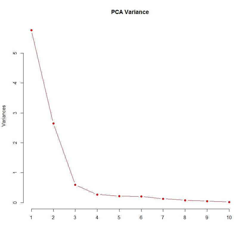
X-axis here represents each of the PCs ranked by their variance. The PCs could be used as features for predicting miles per gallon for our regression analysis. Notice that obtaining PCs are independent of the labels.
Linear Discriminant Analysis:
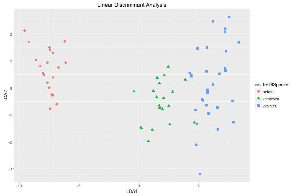
While PCA can be applied to unlabeled data, Linear Discriminant Analysis or LDA is specifically used to find linear combination of features taking into account the classes of the data. The goal here is to maximize the separation between the mean of the classes and minimize the total squared deviation from the means of the individual classes. While PCA retains the variance of all the features while picking the principal component, LDA tries to retain the variance between the features in one class.
 Let's use the iris data to understand what LDA is.

>head(iris)
>train <- sample(1:150, 75)
>lda_model <- lda(Species ~., data = iris, subset=train)

# shows you the mean, used for LDA
> lda_model$means
 Sepal.Length Sepal.Width Petal.Length Petal.Width
setosa 5.020 3.424 1.444 0.248
versicolor 5.936 2.808 4.272 1.320
virginica 6.680 3.048 5.600 2.072

#Predictions on the test data
>lda_pred <- predict(object = lda_model, newdata = iris[-train, ])
>lda_pred$class
>iris_test <- iris[-train, ]
>ggplot() + geom_point(aes(lda_pred$x[,1], lda_pred$x[,2], colour = iris_test$Species, shape = iris_test$Species),
size = 2.5) + ggtitle("Linear Discriminant Analysis") + xlab("LDA1") + ylab("LDA2") + labs(fill = "Species")
Clustering is the method of reducing the dimensionality of the data in an unsupervised manner. This could be done by generating clusters using k-means or other techniques and replacing the features that form a cluster with that cluster's centroid.
Embedded Methods
Certain Machine Learning Algorithms perform variable selection as a part of the training process.
Ranking Features by Importance:
Random Forest is one such algorithm that is not only used for predictions but also for understanding the importance of the variables. In Microsoft R Server, there is a parameter called 'importance' in the randomForest library - rxDForest call that could be set to TRUE to retrieve this information.
 > library(MicrosoftML)
> rf_model <- rxDForest(formula = form, data = mtcars, importance = TRUE )
> rf_model$importance
 IncNodePurity
cyl 91.03235
disp 38.03042
hp 237.59063
drat 0.00000
wt 413.04983
qsec 0.00000
vs 0.00000
am 0.00000
gear 0.00000
carb 11.86286
Certain implementations of Random Forest would let you look at the %IncMSE. %IncMSE is the increase in MSE of the prediction when that particular variable was randomly shuffled or permuted. So, the higher the %IncMSE the more important the variable is as the model output is sensitive to their permutation.
 >rf_model <- randomForest(mpg ~ ., data = mtcars, importance = TRUE)
>rf_model$importance
         %IncMSE IncNodePurity
 cyl   7.0388730     181.07307
 disp 10.5887708     259.59012
 hp    7.8851215     200.42913
 drat  0.8418488      53.52367
 wt    9.7298284     258.87620
 qsec  0.2712216      30.85635
 vs    0.6793172      31.96985
 am    0.4433644      12.17864
 gear  0.4171823      16.94575
 carb  1.2795945      25.76634
> # Plot the IncMSE to visualize the data
> varImpPlot(data_model)
Regularization
When training a model on a specific data set, sometimes the model might fit the data too perfectly. This could lead to generalization errors i.e. a reduced ability to make good predictions on a new set of data. Regularization is the idea of penalizing the loss function by adding a complexity or penalty term (i.e. lambda) - this has proven to avoid over-fitting the data.
There are two methods of regularization that is used with regression – L1 or Lasso and L2 or Ridge regression. L1 penalizes the coefficients by adding a regularization term as the sum of the weights while L2 uses the sum of squares of the weights. L1 Regularization is known to disable irrelevant features leading to sparse set of features. Here and here are some readings on this topic. For a great explanation of Regularization check the 'Linear Model Selection and Regularization' chapter in the book - An Introduction to Statistical Learning.
Summary
To summarize, it's important to spend time extracting, selecting and constructing features based on your data and it's size. It will be valuable in improving the performance of your model. Some features could be selected from a given feature set based on correlation with other predictors or with the label. If you have a small set of features, a quick brute-force approach of attempting different combinations might give you the best set of predictors. If you have a huge feature set especially when compared to the total number of data points - exploring dimensionality reduction techniques or other methods to combine multiple features together might be of help. But ultimately, though some of the methods above would help pick features, it's up to you to evaluate their value in being good predictors.
References
Introduction to Statistical Learning Permutation Feature Importance Using R's glmnet for regularization JMLR Introduction to variable and feature selection R-Blogger's example on using PCA
Comments
- Anonymous
March 23, 2017
Really helpful article! - Anonymous
April 07, 2017
Nice one Madhu! - Anonymous
December 14, 2017
The best article I ever read on feature engineering.Thanks