An Introduction to Machine Learning through Microsoft ML
Guest blog by Christian Hollreiser Microsoft Student Partner at University of Oxford
About Me
Hi! My name is Christian Hollreiser and I am currently reading an MSc in Computer Science at the University of Oxford. My main interest lies in Artificial Intelligence and Machine Learning in particular. I hope to use these fields to find solutions to problems in medical research and healthcare. Linkedin Profile: https://www.linkedin.com/in/christian-hollreiser/
Introduction
In this blog, we will look at how to get started with the Microsoft Azure Machine Learning (Azure ML) tool and demonstrate how it can be used through a mini project. If you are interested in learning more about machine learning, data science and artificial intelligence, Microsoft offer a variety of other course modules as part of their new AI School (see the end of this blog).
We will partially follow the step by step tutorial provided and show how to get started with a hands on machine learning experiment. For a detailed explanation of the mathematical model used in this tutorial, interested readers are referred to the book Machine Learning A Probabilistic Perspective by Kevin Murphy.
Let’s get started!
What is Microsoft Azure Machine Learning?
Azure Machine Learning is an integrated, end-to-end data science and advanced analytics solution. It enables users to prepare data, build models, develop experiments, and deploy models at cloud scale. The main components of Azure Machine Learning are:
• Azure Machine Learning Workbench
• Azure Machine Learning Experimentation Service
• Azure Machine Learning Model Management Service
• Microsoft Machine Learning Libraries for Apache Spark (MMLSpark Library)
• Visual Studio Code Tools for AI
More information about these can be found here. In this blog we will make use of the tools and services in the first two bullet points.
We will install the Azure ML Workbench and configure a new Azure ML Experimentation account. Using these, we will conduct our first experiment in Azure ML on the famous Iris flower data set (or Fisher’s Iris data set - more info here).
For this time, we will look at how to prepare the data and build a simple model. We leave the deployment of the model as an exercise for the reader. Details on this can be found in the tutorial provided on the Microsoft Azure website.
Prerequisites
Before we get started, you need to have a Microsoft Azure subscription in order to be able to use Microsoft Azure ML. You can create a free account here, if you do not have one already.
Creating an Azure Machine Learning Experimentation Account and Installing the Workbench
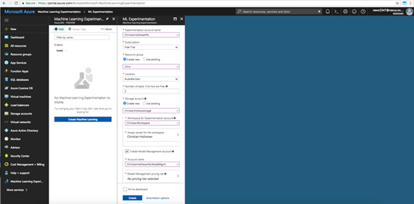
Once you have a Microsoft Azure account, you are ready to create an Azure Machine Learning account. For the purpose of the mini project in this blog, you will need to create an Azure ML Experimentation (preview) account:
1. Log in to your Azure portal and at the bottom of the left-hand side menu select More services.
2. Search for Machine Learning and select the Machine Learning Experimentation option . You may also want to select the star option so that it appears as a favourite in the left-hand side menu (as can be seen in the screenshot below).
3. Next, select + Add in the upper-left corner to set up a new Machine Learning Experimentation account. Enter a unique relevant account name. Fill in the rest of the details as appropriate.
4. Click create when finished. Towards the right side on the Azure portal toolbar, click Notifications (the bell icon). Upon success of the deployment, your new Machine Learning Experimentation account page will open.
5. On your account page, you should be able to see two download options in grey boxes: one for Windows and one for Mac. Select the option that applies to you to download the Azure ML Workbench installer.
6. Once the download is complete, double click the installer AmlWorkbench.dmg from Finder (if you are using Mac OS Sierra or later) or the installer AmlWorkbenchSetup.msi (if you are using Windows 10, Windows Server 2016 or newer).
7. Finish the installation by following the on-screen instructions.
8. You will find the Workbench installed in the Applications directory (if using Mac) or in the directory C:\Users\<user>\AppData\Local\AmlWorkbench (if using Windows).
Note that when installing the Workbench, the necessary components such as Python and Miniconda are also installed.
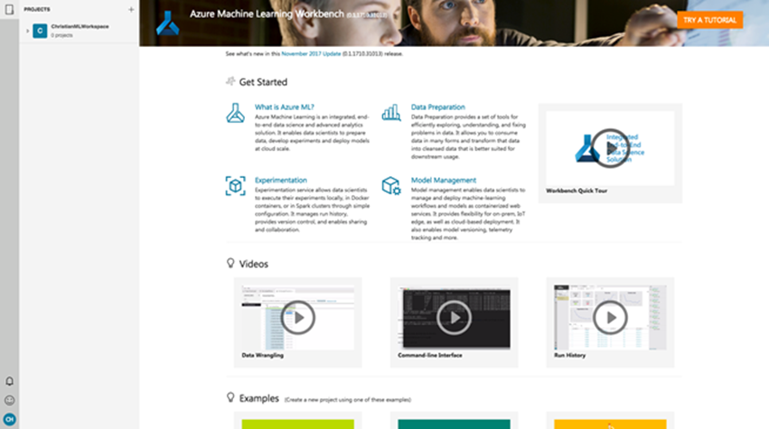
Once successfully installed, launch the Workbench and sign in to it by using the same account that you were using earlier for the Azure portal. Once signed in, the Workbench will automatically open the Experimentation account, which you just created.
You should see it list the workspaces and projects found in that account. As we have not yet created any projects, this will be an empty workspace with zero projects.
Creating a New Project in Azure ML Workbench
Let’s now create your first project using Azure ML:
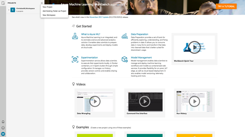
Select the + symbol next to the PROJECTS header in the left panel. Select New Project.
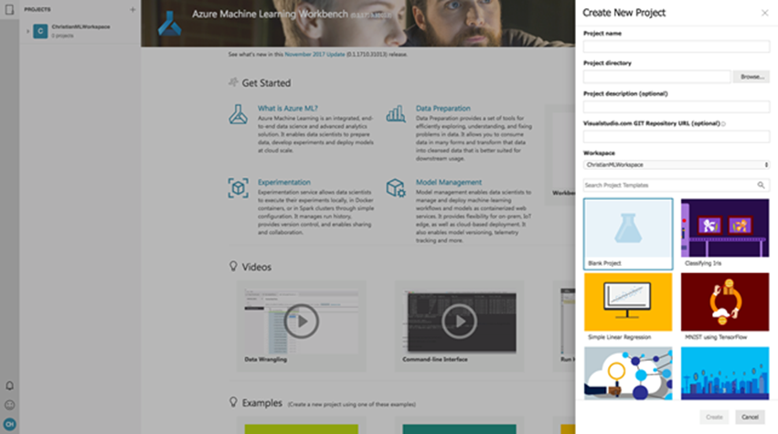
Enter a name for your project, a directory where you want it to be stored, and a (optional) description of the project. Leave the GIT repository free for now. Select a desired workspace: it should select your newly created workspace automatically. Lastly, since we are going to be working with the Iris dataset, select the Classifying Iris template as the project template.
Select Create to finish creating the project.
Upon opening the project, you will see the Project Dashboard. In the side panel to the left of this, you should see five icons:
• The first (house icon) takes you to the dashboard.
• The second (stacked cylinder icon) takes you to the data, where you can manage and prepare your data for the experiment.
• The third (book icon) takes you to the Notebooks.
• The fourth (clock rewind icon) holds your experiment runs. Here you can view all of the details and analysis of the runs.
• The fifth (file icon) stores all the folders and files that are relevant for your project such a code scripts and .csv files which hold raw data.
You are now ready to begin the Classifying Iris experiment.
Classifying Iris Experiment
Data Preparation
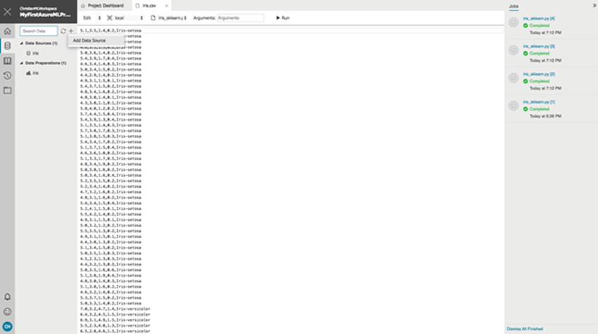
Start by converting the Iris.csv file, containing the raw Iris data, into a data source which can then be prepared for the experiment. To do this, click the data icon in the left panel.
Select the + symbol and click Add Data Source to add a new data source.
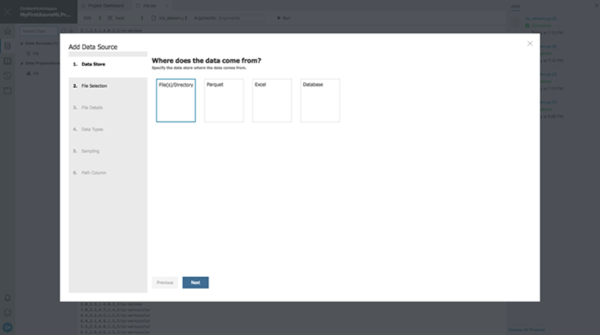
Then, select the box labelled File(s)/Directory for the location of the data and click next.
In the next tab, select Local to search within the project folders and files (described earlier) and select Browse and then File. A window will open, in a directory where you will see the Iris.csv file. Select this file and click open and then Finish.
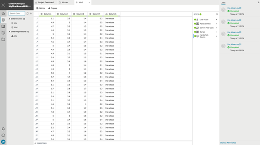
Upon clicking Finish, the new data source iris-1.dsource is created and added to the list of existing data sources. It will open automatically. The data is shown with column headers for each of the four numerical features (Column 1 to Column 4) and for the labels/targets (Column 5).
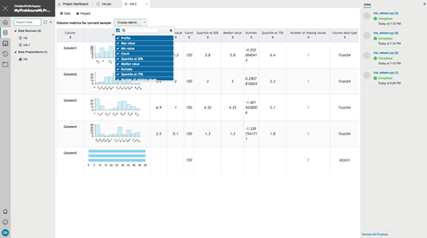
A great feature of Azure ML is the following. If you select the Metrics button just below the tabs panel at the top, you obtain useful statistics about each of the columns in the data source, including a visual histogram for each.
Furthermore, if you select Choose Metric, you can search and filter which statistics you want to view.
You are also able to order the columns by a certain statistic by clicking on the appropriate arrow below the header of the desired statistic in the table.
Next, to prepare this data, select the Prepare button.
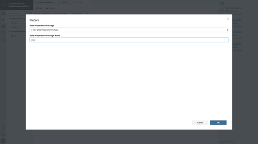
Select + New Data Preparation Package from the drop down menu. Then, name this iris-1 and select OK. This creates the data preparation package iris-1.dprep and opens it in the data preparation editor in a new tab.
You can now prepare the data in this editor. Let’s do some basic preparations:
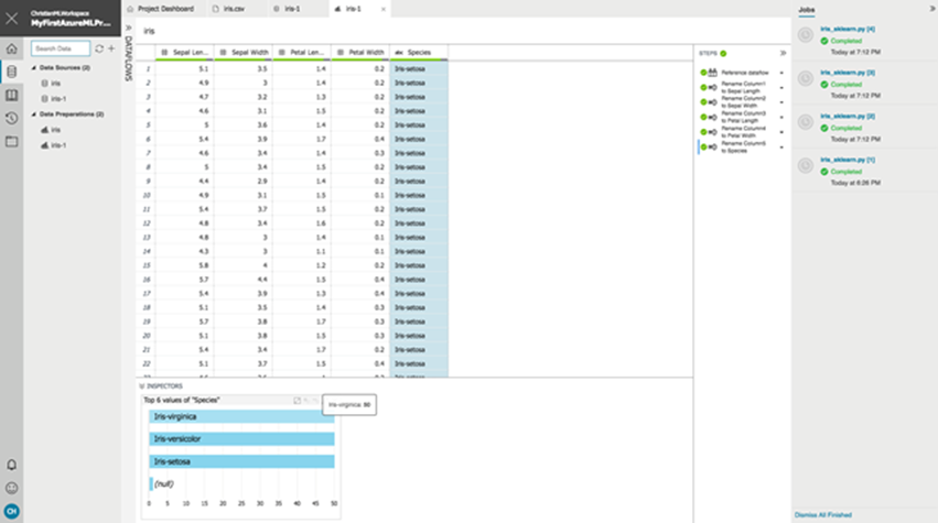
First, rename the column headers to be the respective feature names and label/target name: Sepal Length, Sepal Width, Petal Length, Petal Width and Species.
Second, count distinct values in a column by selecting a column header with the right mouse button and selecting Value Counts.
This opens up the Inspectors window, which displays a histogram of the values. For the Species column, this histogram should have four bars: three for the Iris labels and one for the (null) value. This null value is present due to the data set containing one empty row. To filter out this value, select the bar representing it and then the minus sign filter in the upper right corner of the histogram.
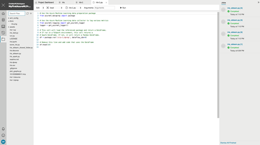
You are now ready to invoke this data preparation package. The Workbench provides the option to automatically generate the code to do this. Close the data preparation editor. Right-click the iris-1.dprep file under the Data Preparations tab in the left panel and select Generate Data Access Code File. This will create a new file named iris-1.py containing the code to invoke the data preparation package that you have constructed as a pandas DataFrame when using Python (see here for more details on the pandas DataFrame).
The last line in the code snippet simply shows an example of the data frame being used, in which the first 10 rows are returned. The purpose of this last part was just to show how one can easily prepare data and generate the code to invoke these preparations.
For the purpose of this blog, we will use a different pre-existing python script (given by the Classifying Iris template) for invoking the data preparation package, in addition to building the model. This script will refer to the pre-existing data preparation file iris.dprep, which is identical to the one which we have shown how to construct. We will cover this in the next section.
Model Building
In this section, you will see how to build a model to model the Iris data, which we prepared in the previous section. For this purpose, we use the logistic regression model for classifying the data (see here or Chapter 8 in Machine Learning: A Probabilistic Perspective by Kevin Murphy).
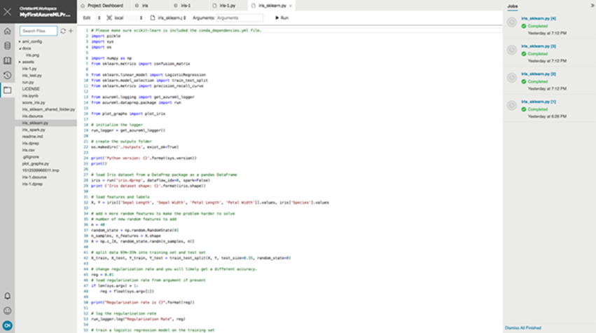
We will make use of the Python script provided in the Classifying Iris template. To view this script, select the Files icon button in the left panel of the Workbench. Next, open the iris_sklearn.py file. Go through this code in order to see how the model is built.
For the interested reader, a useful addition to this code could be to also plot the learning curves, showing the accuracy or mean squared error against incremental amounts of data. This can be done for both the training and test data and the curves can be compared. This gives valuable insight into answering questions such as: does the model overfit? We leave this as an exercise to the reader.
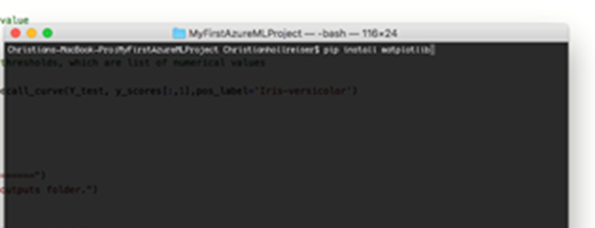
Once you are happy with the code, let’s run the script. In order to be able to run this script successfully, it requires the matplotlib package to be installed. The scikit-learn package was already installed when installing the workbench.
To install the matplotlib package, select File -> Open Command Prompt to open the Azure Machine Learning Workbench CLI (command prompt). Enter the following command.
Once the installation is successful, return to the script in the Azure ML Workbench and locate the toolbar which is above the script and below the tabs.
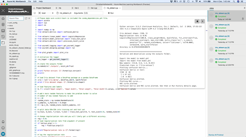
Select local from the first drop down menu (execution environment) , iris_sklearn.py from the second (the script which you want to run), and enter the argument 0.01 in the Arguments box. This value represents the regularization rate for the model.
Next, click Run to run the script with that argument. The job will appear in a pane on the right side of the workbench. Once it has completed, select Completed to view the output.
This shows all of the output that is printed corresponding to the print statements in the script.
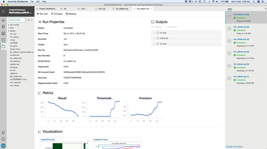
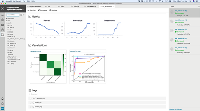
If you close this window and now select iris_sklearn.py[n] (n is the run number), a window opens with information about that run.
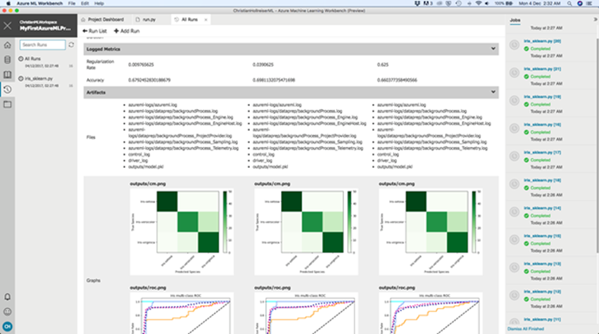
This window displays the properties of the run, the outputs files, the visualisations (if any were coded - here you can see in the script that the confusion matrix and multi-class ROC curve was included), and the Logs.
Now, let’s run the script again with a different regularization rate. You should do this several times with different rates to compare.
Rather than entering them manually like before, a more efficient way to do this would be to write a small Python script that loops over the different rates.
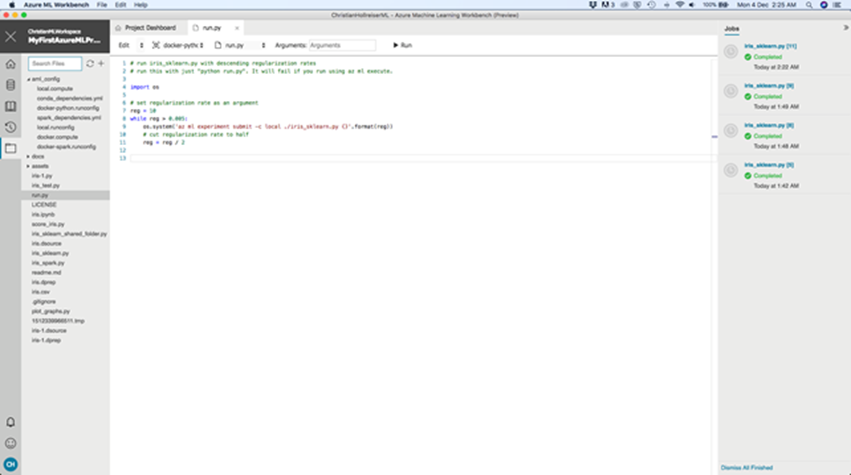
The template that we have been using provides such a script: Open the script run.py, which can be found in the Files section of the workbench.
The script starts with a regularization rate of 10.0 and halves the rate in each of the following runs, until the rate is no less than 0.005.
To run the script, you can use the Azure Machine Learning Workbench CLI (command prompt) which we accessed earlier. Simply enter the following command.
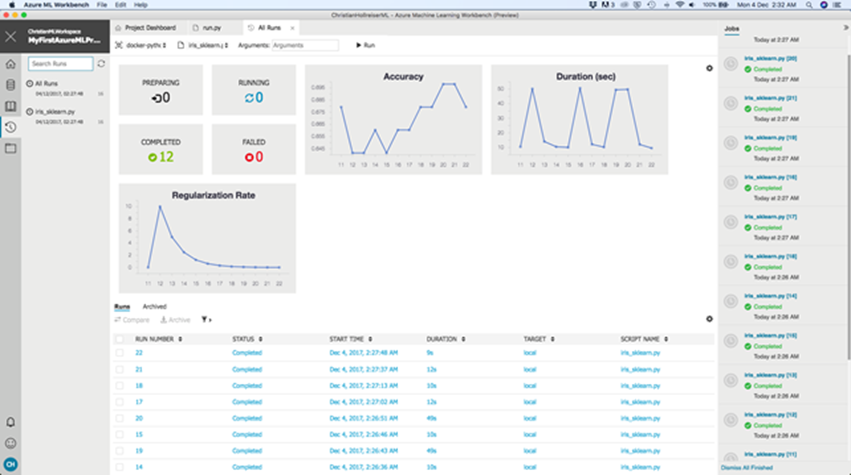
Upon completion, you can compare the runs as follows. Select the Runs icon in the left panel of the workbench and select iris_sklearn.py to view all runs of this script.
We can see how the regularization rate decreased over time in the graph. Note that the first very low rate is from the initial run of the script, that we did with rate 0.01.
In order to compare runs, we can select the desired runs in the list beneath the graphs and select the Compare button.
Here you can compare, side-by-side, the Run Properties (including logged metrics such as the regularization rate) and Visualizations. You can see how the model performs on this dataset with different regularization rates.
Summary
So, you have now seen how to use Azure ML to prepare a data set, build a model and successfully run experiments for that model on that data set. I hope that you have enjoyed following this brief introduction to Machine Learning using Azure ML and that it has given you insight into the large number of possibilities that Azure Machine Learning offers.
What’s next…
• I would encourage you to find other data sets from online resources and try out the tools and methods described above with different models.
• Browse the various other Machine Learning and AI related courses offered by the Microsoft AI School.
Resources and Further Reading
Microsoft AI School: https://aischool.microsoft.com/learning-paths
(Full) Introduction to Machine Learning with Azure ML course:
https://aischool.microsoft.com/learning-paths/4ZYo4wHJVCsUSAKa2EoAk8
Information on Azure ML: https://azure.microsoft.com/en-gb/services/machine-learning-studio/
User guide scikit-learn: https://scikit-learn.org/stable/user_guide.html#user-guide
Book: Machine Learning A Probabilistic Perspective, Kevin Murphy
Comments
- Anonymous
December 07, 2017
that's cool, how do I run the same scenario sans Azure on my local GPGPU-equipped machine?

