Genetic Algorithm, in Reverse Mode
Today I would like to discuss running genetic algorithm… backwards.
Yes, this is possible. Occasionally it is practical, when you need not the best, but the worst solution to a problem.
And I think there are more uses for it. It seems to be helpful with maintaining genetic pool diversity, with avoiding being stuck in local maximum – and therefore with finding better solutions to problems.
Some variations of this idea are apparently known, but not widely. And there is certain bridging between this method and simulated annealing. So I figured it is worth sharing my observations -- and the code accompanying them.
***
Genetic (or evolutionary) algorithms are not first class citizens in the world of optimization methods. The primary reason for that is their ability to make tough problems look deceivingly simple. A basic implementation of a genetic algorithm needs less than a screen of code; the idea behind it is obvious and intuition-friendly. With that, it is very tempting to ignore nature and inherent complexity of a problem being solved and let the CPU cycle, hoping it would eventually crank out a solution.
Only when it fails after millions of seconds one realizes that subtle details rule everything here. How is a solution represented as a vector? What are crossbreeding and mutation strategies? How do you choose the winner and how (or if) do you run a tournament? What do you do to avoid convergence to a sub-optimal maximum? These hyper-parameters are difficult to quantify to enable a systematic search within their space. Yet wrong choices slow things down by orders of magnitude. That’s why genetic algorithms often remain an art (if not a magic) to a large degree -- larger than many alternatives.
Yet they aren't useless. They tolerate poorly defined or implicit fitness functions. They are somewhat less inhibited by the curse of dimensionality. People do solve real problems with them, sometimes quite productively:
They do have their uses, and they are fun to play with.
And one fun aspect is that you can run them backwards.
That’s it, you can replace “good” with “bad” – and run not for the best, but for the worst solution. Besides interesting philosophical implications, this also offers a strategy of dealing with local optima convergence.
***
This issue – converging not to a global, but to a local sub-optimal solution – is inherent to many optimization methods. When a problem has multiple solutions, an algorithm can arrive to *a* solution, and then sit there forever, despite a better solution possibly existing couple valleys away. Steven Skiena described that situation very vividly:
“Suppose you wake up in a ski lodge, eager to reach the top of the neighboring peak. Your first transition to gain altitude might be to go upstairs to the top of the building. And then you are trapped. To reach the top of the mountain, you must go downstairs and walk outside, but this violates the requirement that each step has to increase your score.”
Genetic algorithms are not immune against this. Large body of scientific research addressing it is developed, to name a few examples:
- An Overview of methods maintaining Diversity in Genetic Algorithms
- Maintaining Diversity in Genetic Search
Sometimes the strategy is to run the algorithm multiple times from new random seeds, hoping to converge to a different solution each time. Sometimes people introduce artificial "species pressure" whereas solutions too similar to each other can't cross-breed and converge to the same point. Or they artificially separate the search space into isolated zones. Or punish for staying too close to an already learned local maxima.
***
So how does running algorithm in a “reverse mode” may help with avoiding local maxima?
To illustrate, let’s pretend we are looking for the highest point on the US elevation map:
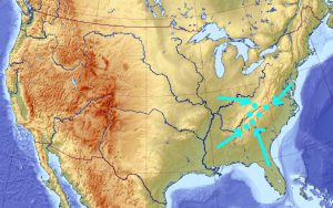
Assume, for a moment, that somehow (maybe because of an unlucky initial placements, maybe because the map is more complex than this) all genetic pool solutions congregated around a wrong local maximum of Appalachian Mountains:
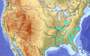
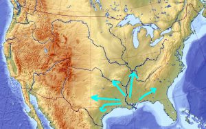
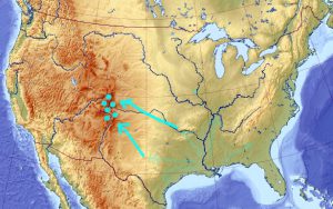
[Important: the arrows do not imply continuous movement. Genetic algorithm does not work like a gradient descent. The arrows serve purely illustrational purposes of indicating (most likely discontinuous) state transitions]
What happens if you switch the evolution sign at this moment? When the least fit wins, and the worst solution is rewarded, the genetic pool starts running away from the local maximum, initially in all directions:
That diversifies it. Soon, the pool may have very little in common with the solution it initially described. After a while, it may even converge to a local minimum, which I would guess is near the Mississippi delta (though there is no point necessarily in keeping the evolution “in reverse” that long enough):
Now let’s flip the sign of the evolution back to normal. Again, the solutions will start scattering away in all direction from the local minima:
And, if some of them arrives to a point elevated enough, eventually everyone would re-converge there:
In a two-dimensional case, this is almost trivial. But in higher dimensionality, where mountains are more difficult to discover, these fourth-and-back cycles may need to continue until you are happy with the solution. Or at least happier than in the beginning -- I'm not promising miracles here :))
Why would this work better than restarting each time from a random seed?
It may not always do, though my testing suggests that sometimes it does. The main benefit here is in having the control over the degree of the digression. If other maximum is expected far away or nearby, the backwards-evolution can run for longer or shorter period, as needed. In that respect, this approach is similar to simulated annealing which is able to adjust annealing schedule to throw just the right degree of chaos into the computation.
But all the above are just my expectations. Would they work in practice?
Lets find out by playing it against a toy problem that is easy to visualize.
Welcome the Scary Parking Lot Problem.
***
Imagine that this is a map of a parking lot at night. There are a few lights producing illuminated patches here and there, and the rest of it is mostly dark:
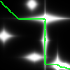
The darker the area, the scarier it is in it. Our goal is to find the least scary path from the top left to the bottom right. To be precise, we want to minimize the integral of Fear = 1/(1 + Brigthness) along the path. If asked, I would’ve probably charted it like this:
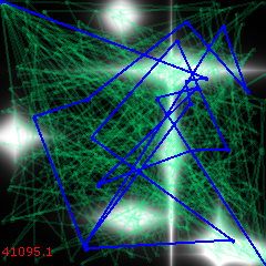
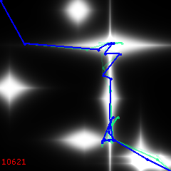
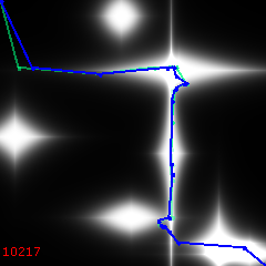
This problem is well suited for genetic algorithm. Encode a path as a sequence of <x, y> points. A genome is represented then as a sequence <x0, y0, x1, y1, ..., xN, yN> (I used N = 20). Initialize the pool randomly with K =16 instances colored in green (blue shows the best solution found so far), and kick off the algorithm.
Iteration 0:
In just 500 iterations, the algorithm already hints at a decent approximation:
1000 iterations:
4000:
By 9000, it is mostly straightening out small knots:
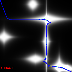
18000 generations – final or nearly final:
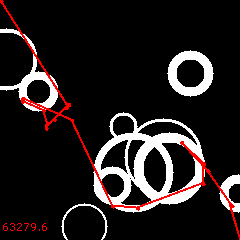
[The red figure at the bottom left is the "cost", or the total fear factor, of the solution -- the smaller, the better].
***
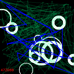
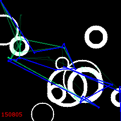
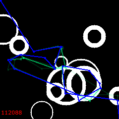
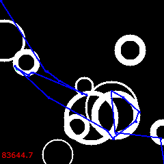
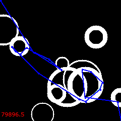
I tried it on a few dozen randomly generated “parking lots” and discovered that genetic algorithm solves this problem so well that it is actually difficult to find a field that would produce a grossly imperfect result. It took quite many experiments until I discovered this “foam bubbles” setup with intentionally harsh contrast and narrow illuminated zones. Constantly forced to make difficult right-or-left choices, and having no gradient feedback, the algorithm responded with some mistakes here.
Start:
500 iterations:
2000:
7000:
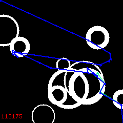
18000 (final):
The solution is stuck. Wrapped around a bubble, it won't change to anything better no matter how long you run it. Not coincidentally, it has also lost its genetic diversity.
***
Now let’s try to untangle it by enabling the reversals. Every 6000 iterations we will put the evolution in the “backwards mode” for 210 steps.
For the first 6000 generations it is the same game, converging to the already familiar solution:
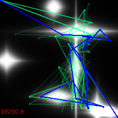
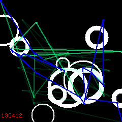
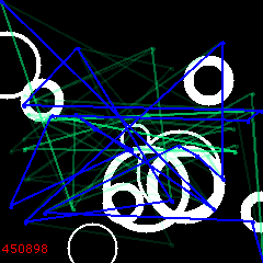
But then, at 6000, the reversal begins. “Bad” solutions are in favor now. Lets’ watch how they develop, spreading away from the original path.
6100:
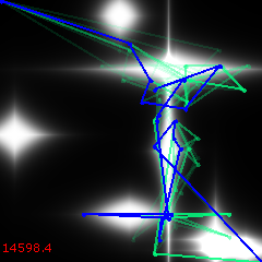
6200:
At 6210 the sign changes back to normal and we start re-converging – to a different maximum this time!
At 1200:
After 12000, another reversal cycle follows, ending up with the 3rd solution at 18K:
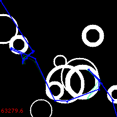
Of all three, the 2nd is the best:
Its cost is 63279.6. It is still not perfect, but the control (without reversals) was 79896.5. The new solution is 20.8% cheaper!
***
But maybe this works just for this one parking lot?
Let’s repeat the experiment 40 times with different “bubble sets”, each randomly generated:
| Control (18K iterations) | Experiment (18K iterations, with 2 reversals 210 steps each) | |
|---|---|---|
| Average cost of the best solution relative to a random path | 0.13448 | 0.11605 |
| Standard deviation | 0.034179 | 0.024659 |
| Student t-score of the improvement | N/A | 2.76637863954974 |
| How many times the solution found was better than control? | N/A | 30 (out of 40) |
A one-sided t-score of 2.77 with 40 degrees of freedom corresponds (https://en.wikipedia.org/wiki/Student%27s_t-distribution#Table_of_selected_values) to roughly 99.5% chance that the difference is not accidental. In other words, that the experiment with reversals indeed performed better than the same 18K iterations straight. And for 30 parking lots (out of 40), the solution found was better than the control.
How does it compare to simply doing three runs with 6K steps, each starting from a random seed, and then selecting the best solution? It is about the same, or maybe very slightly better. Restarts from the scratch produced an improvement t-score of 2.5538656109400, with 24 runs out of 40 doing better than control.
***
Finally, why 210 reversal steps? Why not more or less?
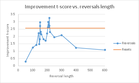
This is where the power of the idea materializes. Reversals let you control their duration – and adjust it as needed for the task being solved. By playing with those durations, I produced the following plot of improvement t-score (relative to the control):
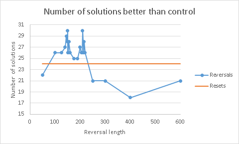
Blue curve are the results with reversals, orange is the result of random reset (for fixed RNG seeding). Obviously, there is fluctuation here, so I can’t strictly say that reversals are better than random resets. But it does not take away the fact that reversals produced some solutions better than anything else tried did.
Finally, here is another plot, showing the number of “parking lots” where solutions with reversals or random reset were better than control:
***
So, is this method a magic bullet? Probably not. It is just a tool, among many other invented by people to deal with practical problems. But maybe it would be helpful for some.
To summarize:
- Reversing genetic algorithm during its run is possible
- …at least, for finding deliberately bad “anti-solutions” to a problem
- …or simply for fun
- More importantly, sometimes it can help combat the loss of pool’s genetic diversity
- Short controlled reversals can produce solutions notably better than those from simple uninterrupted runs of the same duration
- They are at least comparable in quality to solutions achieved by restarting the algorithm from scratch the same number of times as the number of reversals
- Duration and frequency of reversal cycles are controllable numeric parameters that could be adjusted to suit a problem at hands

