Cardinality Estimation for Correlated Columns in SQL Server 2016
Cross post with aka.ms/sqlserverteam
When we introduced the new CE back in SQL Server 2014, several changes were done regarding the assumptions of the model. These changes were introduced because the vast potential for variations in data distribution, volume and query patterns, made some of the model assumptions not applicable.
The 4 assumptions for the pre-2014 model were:
- Independence: Data distributions on different columns are assumed to be independent, unless correlation information is available and usable.
- Uniformity: Distinct values are evenly spaced and that they all have the same frequency. More precisely, within each histogram step, distinct values are evenly spread and each value has same frequency.
- Containment (Simple) : Users query for data that exists. For equi-join of two tables, we factor in the predicates selectivity in each input histogram before joining histograms and come up with the JOIN selectivity.
- Inclusion: For filter predicates where Col = Const, the constant is assumed to actually exist for the associated column. If a corresponding histogram step is non-empty, one of the step’s distinct values is assumed to match the value from the predicate.
A few of those assumptions changed in SQL Server 2014 CE, namely:
- Independence becomes Correlation: The combination of the different column values are not necessarily independent. This may resemble more real-life data querying.
- Simple Containment becomes Base Containment: Users might query for data that does not exist, so we use probabilistic approach. For equi-join of two tables, we use the base tables histograms to come up with the JOIN selectivity, and then factor in the predicates selectivity.
For Base Containment, there was a trace flag (2301) to enable it in prior versions – see the article Tuning options for SQL Server when running in high performance workloads.
You can read more about CE changes in the white paper Optimizing Your Query Plans with the SQL Server 2014 Cardinality Estimator.
For correlated columns in the 2014 CE, to derive cardinality we need to sort the filters according to their density, where the smallest density value is first. Since the density is expressed in a range between 0.xxxx and 1 the smaller values means lower density, better selectivity or more different values. We then use only the first four most selective filters to calculate the combined density, using Exponential Backoff, expressed like:
p0 × p11⁄2 × p21⁄4 × p31⁄8 × Tc
This hasn’t changed per se in the 2016 CE, but there is a relevant difference. While in the 2014 CE we always used the single column statistics for each of the predicate columns, in 2016 CE, if multi-column statistics over the predicate columns are available, those will be used to derive estimations with a different calculator. Allow me to demonstrate using AdventureWorksDW2014.
First we need to set the database compatibility level to 120, to force usage of the 2014 CE to see what statistics are loaded and used in SQL 2014:
 ALTER DATABASE [AdventureWorksDW2014] SET COMPATIBILITY_LEVEL = 120
GO
The create a multi-column statistics object over the columns we’ll be using as predicates:
 CREATE STATISTICS [StatDemo] ON [dbo].[FactInternetSales] (CurrencyKey,SalesTerritoryKey)
GO
Now create a xEvent session to track the query_optimizer_estimate_cardinality event:
 CREATE EVENT SESSION [XeNewCE] ON SERVER
ADD EVENT sqlserver.query_optimizer_estimate_cardinality(
    ACTION(sqlserver.sql_text)),
ADD EVENT sqlserver.query_optimizer_force_both_cardinality_estimation_behaviors
ADD TARGET package0.event_file(SET filename=N'H:\Demo\XeNewCE.xel',max_file_size=(50),max_rollover_files=(2))
GO
Let’s start the session:
 USE AdventureWorksDW2014
GO
DBCC FREEPROCCACHE
GO
ALTER EVENT SESSION [XeNewCE] ON SERVER STATE = START
GO
Run the query and stop the session to look at the events:
 SELECT * FROM FactInternetSales
WHERE CurrencyKey = 98 AND SalesTerritoryKey = 10
GO
ALTER EVENT SESSION [XeNewCE] ON SERVER STATE = STOP
GO
Now open the session file, and take a look at the calculator field. As expected, using Exponential Backoff and we see the selectivity derived for each predicate column:
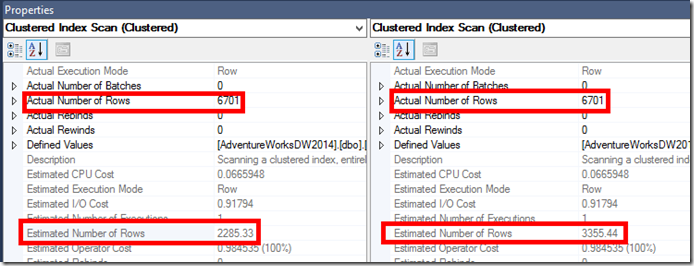
If you see the stats_collection field, the derived cardinality is shown at 2285.33 which is the result of the Exponential Backoff derivation (0.112 * SQRT(0.114) * 60398):
Next, change the database compatibility level to 130, to force usage of the 2016 CE and see what statistics are loaded now.
 ALTER DATABASE [AdventureWorksDW2014] SET COMPATIBILITY_LEVEL = 130
GO
Let’s start the session again:
 DBCC FREEPROCCACHE
GO
ALTER EVENT SESSION [XeNewCE] ON SERVER STATE = START
GO
Run the same query and stop the session to look at the events:
 SELECT * FROM FactInternetSales
WHERE CurrencyKey = 98 AND SalesTerritoryKey = 10
GO
ALTER EVENT SESSION [XeNewCE] ON SERVER STATE = STOP
GO
We can see a different calculator in use, using a multi-column statistic we created on the predicate columns CurrencyKey and SalesTerritoryKey. Individual stats are still available if required:
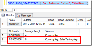
And in the stats_collection field, the derived cardinality is shown at 3355.44 which is the result of simple density calculation (0.05555556 * 60398):
Just have a look at the density for the predicate columns:
The practical outcome with this query is still the same for this case, as seen in the scans chose below, but generally, more accurate estimations will allow better plans to be used.
Pedro Lopes (@sqlpto) - Program Manager


