Configure the model to generate insights
In this exercise, you assume the role of Jessie and configure the Frequently bought together model to generate insights by using a predeployed notebook.
The notebook includes cells that describe how data is processed to provide the required output. To complete this exercise, follow these steps:
In a new Incognito or InPrivate browsing session, sign in to your Microsoft Power BI home page with the credentials of Jessie Irwin.
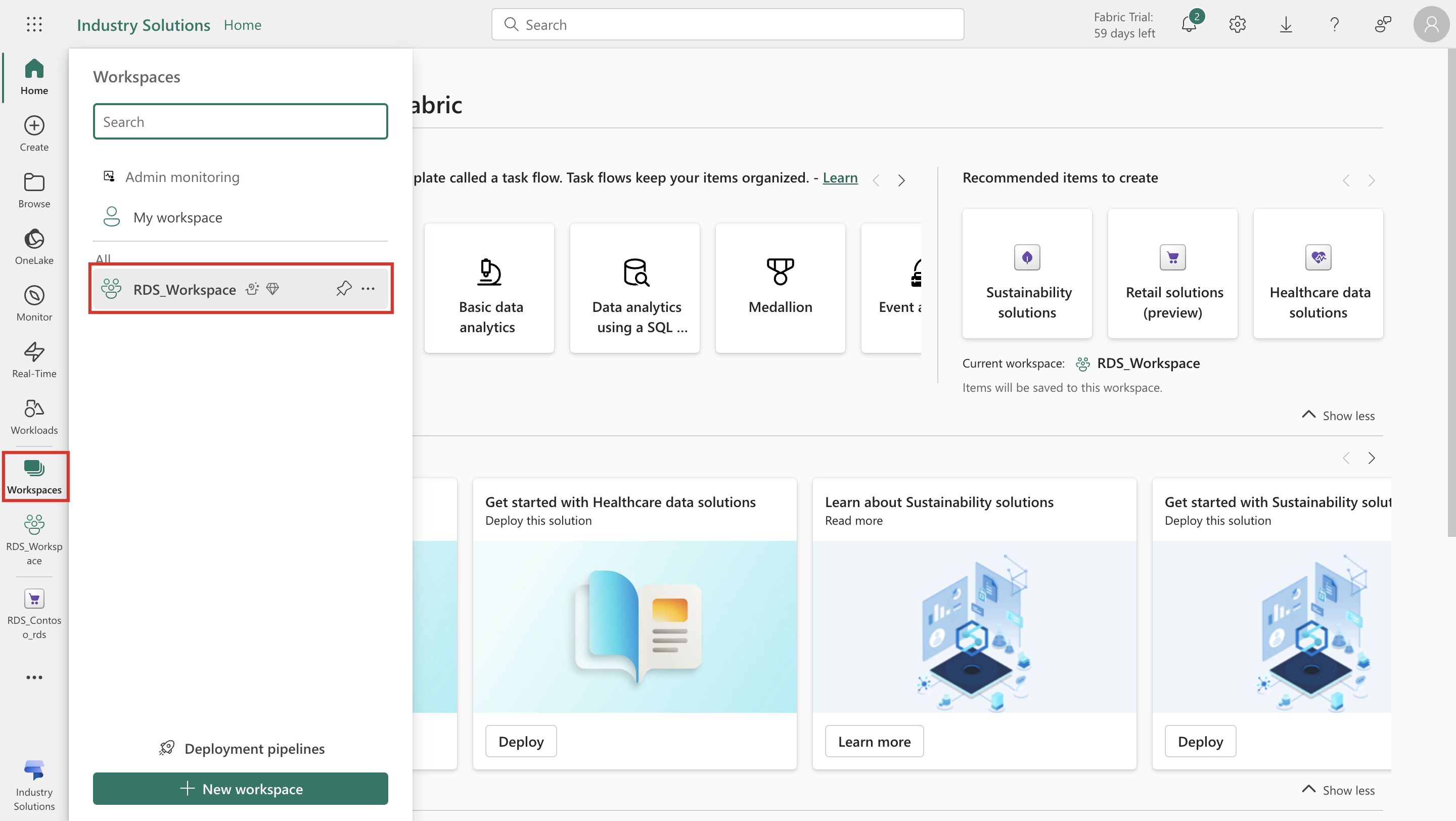
From the left navigation, select Workspace > RDS_Workspace.
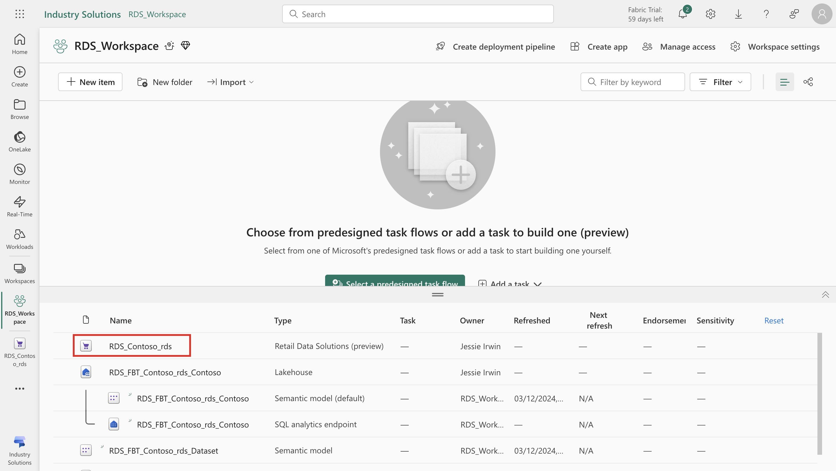
Select Retail Data Manager or RDS_Contoso_rds.
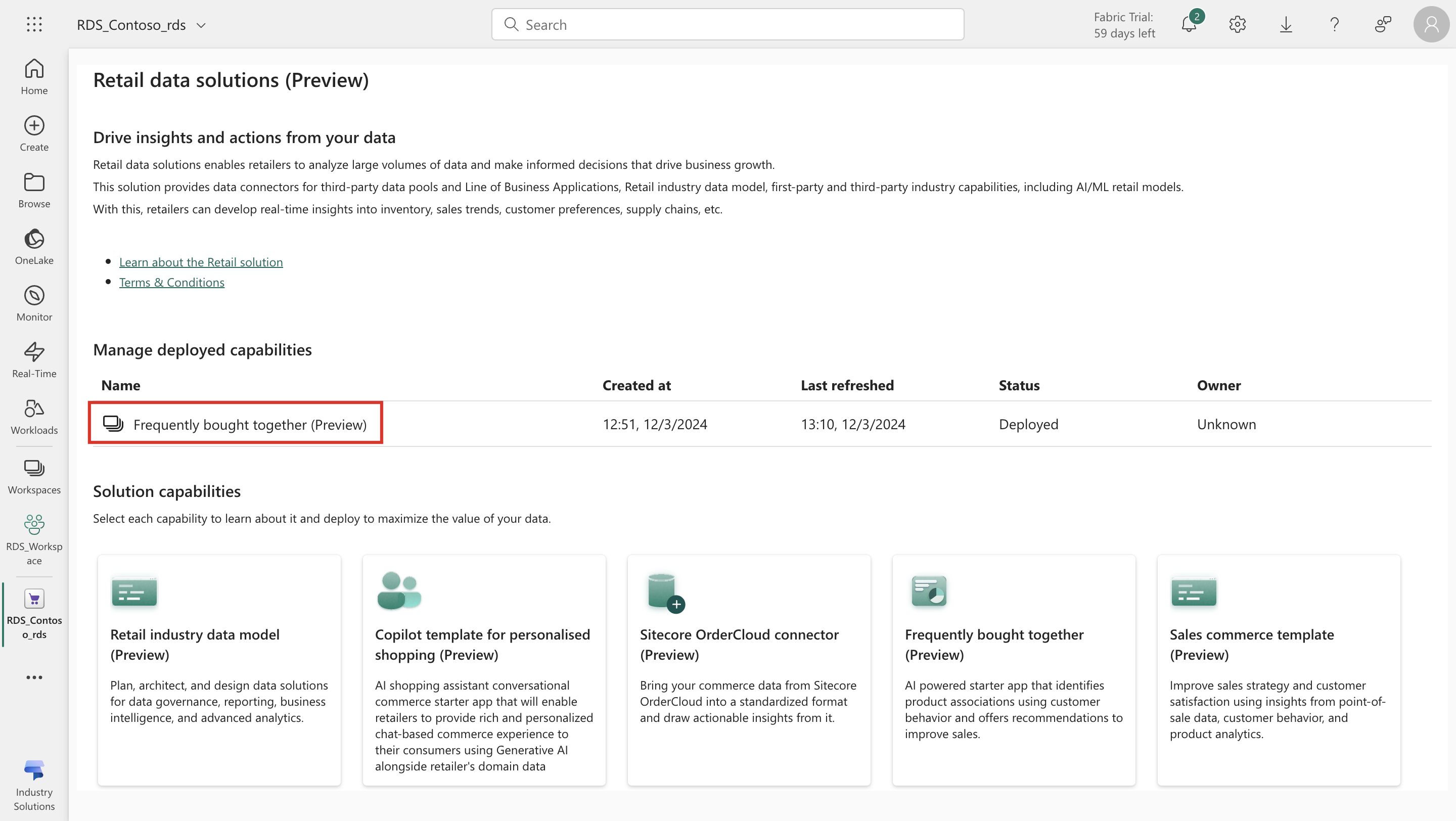
Select Frequently bought together (Preview) under Manage deployed capabilities.
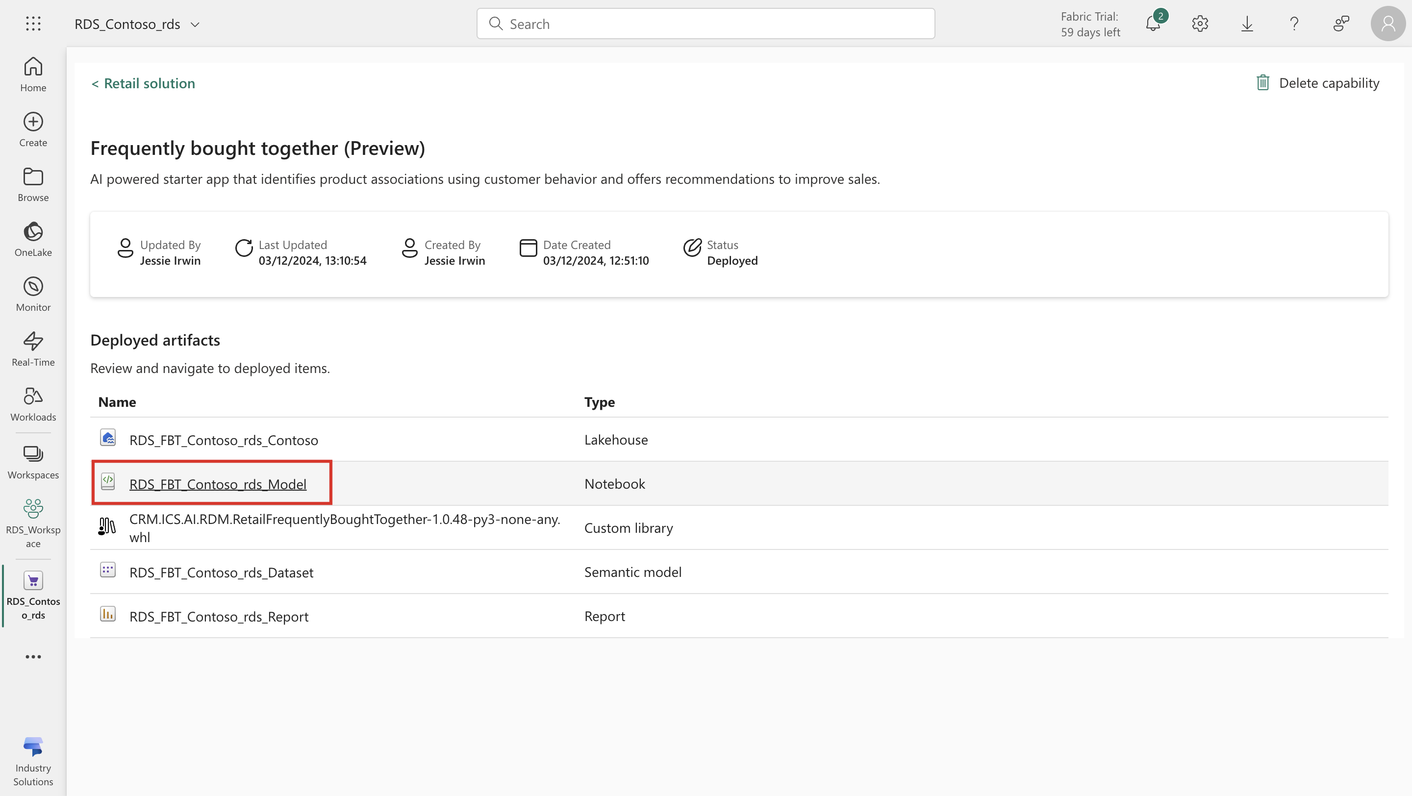
Open the Deployed artifacts panel and select the RDS_FBT_Contoso_rds_Model notebook.
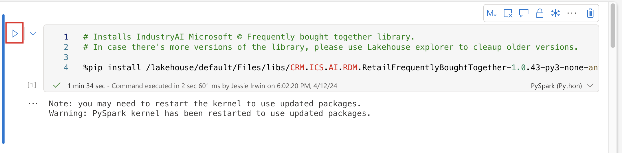
Select the run cell button to the left of the cell to run the first cell. Running this cell would ensure that the Frequently bought together library is installed.
Now in the Frequently bought together library, run each cell in the following recommended sequence. If you run the cells in a different sequence, the notebook fails. The ensuing sections describe each step in detail:


Step 1: Import libraries
The first step in the process is Import libraries, where you import the necessary libraries for the notebook. You don't need to make changes in this step. Select Run to run the cell.

Step 2: Initialize spark configs, logger, and checkpointer
In this step, you initialize the spark configs, logger, and checkpointer objects that you use for the notebook implementation.
You can initialize the logger in two different ways:
Set up to write logs to the notebook cell outputs. This behavior is the default.
Set up to write logs to a Microsoft Azure Application Insights workspace. For this approach, you need the connection_string of the Application Insights workspace. The system generates a Run ID and then shows it in the cell's output. You can use the Run ID to query logs in the Application Insights workspace.
You can use the checkpointer to sync Spark implementation and to avoid potential generation of duplicated keys. You must provide a path that you plan to use as a working directory. The name of the variable is checkpoint_dir. The directory must be within the files section of the Lakehouse, that is, it needs to start with "Files/".
Select Run to run the cell.

Step 3: Connect to the Lakehouse and read input tables
In this step, you connect to the Lakehouse and read input tables that are required for the model. You can read the input tables from one of the following three options:
The pinned Lakehouse of the notebook, which contains the sample data. This option is the default.
Lakehouses that are connected to the notebook. You can select the Lakehouse from a dropdown menu.
Another Lakehouse that isn't connected to the notebook. You need to provide the full path to the Lakehouse.
For more information, see Input data for Frequently bought together.
Select Run to run the cell.

Step 4: Define analysis periods for the model
The notebook allows you to run the model on multiple time periods, which can help you capture the seasonality and changes in customer behavior, product portfolio, and product positioning over time. Additionally, you can compare the results of different time periods by using the out-of-the-box dashboard.
To define a time period, use the add_analysis_period function. Make sure that you define the analysis periods in the duration of the input data. You can log the duration of the input data (maximum and minimum transactions timestamp) in the cell's output. You can define up to five time periods. The TimePeriods table stores the reference keys for the periods.
Select Run to run the cell.

Step 5: Preprocess input data
After defining analysis periods for the model, you can preprocess input data. This step joins the input dataframes to create a point-of-sale (POS) dataset, which the model uses to generate insights. You don't need to make changes in this step.
The output of this step includes the following dataframes:
purchases - The purchases POS dataframe contains information about the purchases that customers make, such as retail entity ID, product ID, product list price amount, quantity, and visit timestamp. You can create this dataframe by joining the Visit, ShopperSession, ShopperSessionTransaction, and TransactionLineItem tables.
time_periods - This dataframe contains the analysis periods that you define in the previous step. You can use these periods to split the data and run the model on each period.
retail_entities - This dataframe contains the retail entity IDs and their information. A retail entity can be an individual store or a retailer. You can use these entities to run the model on a store level or a retailer level.
Select Run to run the cell.

Step 6: Define model parameters and run the model
In this step, you define model parameters and run the model. You can set the following model parameters to fine-tune the model results:
Parameter name - min_itemset_frequency
Description - Minimal number of purchases of item sets (collection of two products bought together) to be considered in the analysis of the model.
Value type - integer
Default value - 3
Required - true
Permitted values - >=1
Parameter name - max_basket_size
Description - Maximum number of items in one basket. If the number of items in the basket exceeds the default value, the basket is trimmed. The product with the lowest sales in the dataset is trimmed first.
Value type - integer
Default value - 20
Required - true
Permitted values - >=1
Parameter name - chi_2_alpha
Description - Statistical significance parameter. You use this parameter to determine whether a pair of products that are associated together is meaningful and statistically significant. If a pair of products scores less than the parameter value, they're flagged in the Chi2IsSignificant field on the RuleAttributes table.
Value type - float
Required - false
Default value - 0.05 percentile
Permitted values range - 0-1
When you finish setting model parameters, the system writes the data to the output tables. You have three options to define which Lakehouse to write to.
Select Run to run the cell.
Step 7: Create Power BI dashboard tables
In this step, you create Power BI dashboard tables. Similar to the Connect to Lakehouse and read input tables section, there are three methods of writing outputs to Fabric.

After you finish creating the Power BI dashboard tables, the system writes data to the Lakehouse. Select Run to run the cell.
For more information, see output data tables.
Step 8: Create a view with 'Excellent association' only
'Excellent association' is a classification that suggests a strong and statistically significant relationship between the products based on the criteria set in the SQL code. 'Excellent association' is derived from the StrengthOfAssociation column that is populated based on conditional statements in the SQL code. This logic categorizes the strength of association between products based on the values of RuleQualityCategoryId and IsSignificant columns in the FBT table.
'Excellent association' refers to cases where RuleQualityCategoryId is 2 (which might signify a high-quality association rule) and IsSignificant is 1 (which might indicate that the association is statistically significant).
If IsSignificant is 0, it means that although the rule category might be considered excellent, the significance might be limited due to insufficient data.
In this step, you create a view with 'Excellent association' only. This step makes the products symmetrical. Essentially, if Product1=A and Product2=B, then you need to create a symmetrical record as Product1=B and Product2=A. You should query A and B separately.
Select Run to run the cell.
Step 9: Power BI dashboard table parameters
You can use the num_top_associated_products parameter to configure the number of top associated products to display in the Power BI dashboard for each product.
Description - Maximum number of associated products for each product to be shown in the Power BI dashboard. Returns top products that the Combination Rank field sorts.
Value type - integer
Required - false
Default value - 5
Permitted values range - 1-10
Select Run to run the cell.
Step 10: Create views
You can create views from the previous information, where you calculate purchase amounts and quantities as weekly averages.
This step replicates data for each product criteria/group that you want to view separately. You can complete this step by ranking each store/retailer, time period, and currency.
All items (if Frequently bought together is with another item)
10 highest Frequently bought together revenues (main + Frequently bought together)
10 lowest Frequently bought together revenues (main + Frequently bought together)
Best seller in main item revenue
Lowest seller in main item revenue
The view represents main items (Product1) for each store/retailer, time period, currency, and product criteria with its weekly revenue, quantity, and sum of all Frequently bought together products' revenue.
Select Run to run the cell.
Step 11: Create a table that the Power BI dashboard consumes
The table that you create in this last step is directly consumable without the need for creating other Power BI measures or calculated columns.
Three types of records exist according to TableColProductGroupType:
Type=1: TableColProductGroup="Group N" - This record represents the main item that's part of the Frequently bought together dashboard table.
Type=2: TableColProductGroup="Main product" - This record also represents the main item that's part of the Frequently bought together dashboard table as another record.
Type=3: TableColProductGroup="FBT product" - This record represents the associated item with the main product.
Select Run to run the cell.
Congratulations! Now you have completed the cleanup of data and have created the Power BI report with appropriate filters using the notebook. You can use this report to derive actionable insights.