Object detection using Fast R-CNN
Table of Contents
- Summary
- Setup
- Run the toy example
- Run Pascal VOC
- Train CNTK Fast R-CNN on your own data
- Technical details
- Algorithm details
Summary
This tutorial describes how to use CNTK Fast R-CNN with BrainScript and cntk.exe. Fast R-CNN using the CNTK Python API is described here.
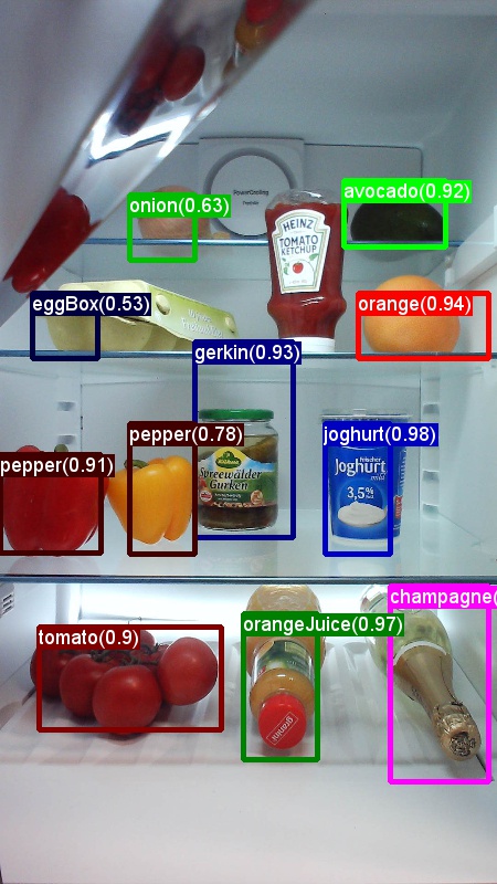
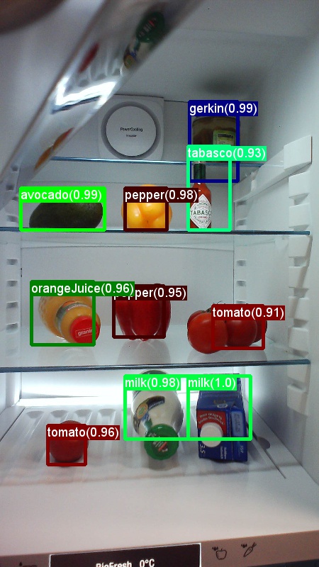
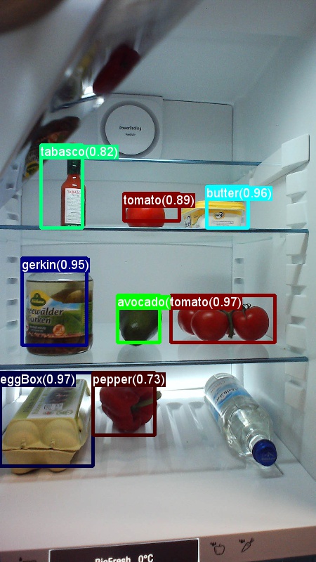
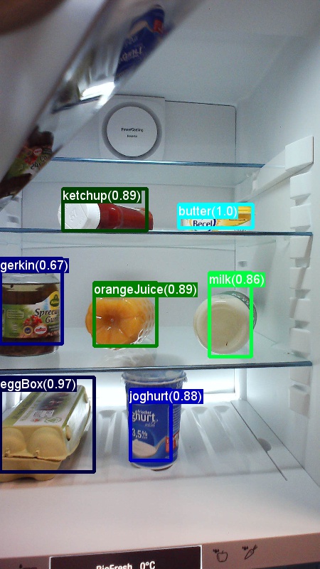
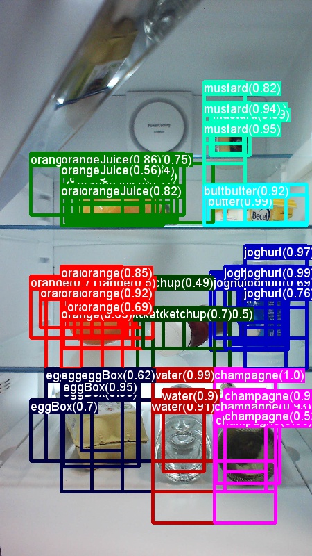
The above are examples images and object annotations for the grocery data set (first image) and the Pascal VOC data set (second image) used in this tutorial.
Fast R-CNN is an object detection algorithm proposed by Ross Girshick in 2015. The paper is accepted to ICCV 2015, and archived at https://arxiv.org/abs/1504.08083. Fast R-CNN builds on previous work to efficiently classify object proposals using deep convolutional networks. Compared to previous work, Fast R-CNN employs a region of interest pooling scheme that allows to reuse the computations from the convolutional layers.
Additional material: a detailed tutorial for object detection using CNTK Fast R-CNN with BrainScript (including optional SVM training and publishing the trained model as a Rest API) can be found here.
Setup
To run the code in this example, you need a CNTK Python environment (see here for setup help). Further you need to install a few additional packages. Go to the FastRCNN folder and run:
pip install -r requirements.txt
Known issue: to install scikit-learn you might have to run conda install scikit-learn if you use Anaconda Python.
You will further need Scikit-Image and OpenCV to run these examples.
Please download the corresponding wheel packages and install them manually. On Linux you can conda install scikit-image opencv.
For Windows users, visit http://www.lfd.uci.edu/~gohlke/pythonlibs/, and download:
- Python 3.5
- scikit_image-0.12.3-cp35-cp35m-win_amd64.whl
- opencv_python-3.2.0-cp35-cp35m-win_amd64.whl
Once you download the respective wheel binaries, install them with:
pip install your_download_folder/scikit_image-0.12.3-cp35-cp35m-win_amd64.whl
[!NOTE]: if you see the message No module named past when running the scripts please execute pip install future.
This tutorial code assumes you are using 64bit version of Python 3.5 or 3.6, since the required Fast R-CNN DLL files under utils are prebuilt for those versions. If your task requires the use of a different Python version, please recompile these DLL files yourself in the correct environment (see below).
The tutorial further assumes that the folder where cntk.exe resides is in your PATH environment variable. (To add the folder to your PATH you can run the following command from a command line (assuming the folder where cntk.exe is on your machine is C:\src\CNTK\x64\Release): set PATH=C:\src\CNTK\x64\Release;%PATH%.)
Pre-compiled binaries for bounding box regression and non maximum suppression
The folder Examples\Image\Detection\FastRCNN\BrainScript\fastRCNN\utils contains pre-compiled binaries that are required for running Fast R-CNN. They versions that are currently contained in the repository are Python 3.5 and 3.6, all 64 bit. If you need a different version you can compile it following these steps:
git clone --recursive https://github.com/rbgirshick/fast-rcnn.gitcd $FRCN_ROOT/libmake- Instead of
makeyou can runpython setup.py build_ext --inplacefrom the same folder. On Windows you might have to comment out the extra compile args in lib/setup.py:
ext_modules = [ Extension( "utils.cython_bbox", ["utils/bbox.pyx"], #extra_compile_args=["-Wno-cpp", "-Wno-unused-function"], ), Extension( "utils.cython_nms", ["utils/nms.pyx"], #extra_compile_args=["-Wno-cpp", "-Wno-unused-function"], ) ]- Instead of
copy the generated
cython_bboxandcython_nmsbinaries from$FRCN_ROOT/lib/utilsto$CNTK_ROOT/Examples/Image/Detection/fastRCNN/utils.
Example data and baseline model
We use a pre-trained AlexNet model as the basis for Fast-R-CNN training. The pre-trained AlexNet is available at https://www.cntk.ai/Models/AlexNet/AlexNet.model. Please store the model at $CNTK_ROOT/PretrainedModels. To download the data please run
python install_grocery.py
from the Examples/Image/DataSets/Grocery folder.
Run the toy example
In the toy example we train a CNTK Fast R-CNN model to detect grocery items in a refrigerator.
All required scripts are in $CNTK_ROOT/Examples/Image/Detection/FastRCNN/BrainScript.
Quick guide
To run the toy example, make sure that in PARAMETERS.py dataset is set to "Grocery".
- Run
A1_GenerateInputROIs.pyto generate the input ROIs for training and testing. - Run
A2_RunWithBSModel.pyto train and test using cntk.exe and BrainScript. - Run
A3_ParseAndEvaluateOutput.pyto compute the mAP (mean average precision) of the trained model.
The output from script A3 should contain the following:
Evaluating detections
AP for         avocado = 1.0000
AP for          orange = 1.0000
AP for          butter = 1.0000
AP for       champagne = 1.0000
AP for          eggBox = 0.7500
AP for          gerkin = 1.0000
AP for         joghurt = 1.0000
AP for         ketchup = 0.6667
AP for     orangeJuice = 1.0000
AP for           onion = 1.0000
AP for          pepper = 1.0000
AP for          tomato = 0.7600
AP for           water = 0.5000
AP for            milk = 1.0000
AP for         tabasco = 1.0000
AP for         mustard = 1.0000
Mean AP = 0.9173
DONE.
To visualize the bounding boxes and predicted labels you can run B3_VisualizeOutputROIs.py (click on the images to enlarge):
Step details
A1: The script A1_GenerateInputROIs.py first generates ROI candidates for each image using selective search.
It then stores them in a CNTK Text Format as input for cntk.exe.
Additionally the required CNTK input files for the images and the ground truth labels are generated.
The script generates the following folders and files under the FastRCNN folder:
proc- root folder for generated content.grocery_2000- contains all generated folders and files for thegroceryexample using2000ROIs. If you run again with a different number of ROIs the folder name will change correspondingly.rois- contains the raw ROI coordinates for each image stored in text files.cntkFiles- contains the formatted CNTK input files for images (train.txtandtest.txt), ROI coordinates (xx.rois.txt) and ROI labels (xx.roilabels.txt) fortrainandtest. (Format details are provided below.)
All parameters are contained in PARAMETERS.py, for example change cntk_nrRois = 2000 to set the number of ROIs used for training and testing. We describe parameters in the section Parameters below.
A2: The script A2_RunWithBSModel.py runs cntk using cntk.exe and a BrainScript config file (configuration details).
The trained model is stored in the folder cntkFiles/Output of the corresponding proc sub-folder.
The trained model is tested separately on both the training set and the test set.
During testing for each image and each corresponding ROI a label is predicted and stored in the files test.z and train.z in the cntkFiles folder.
A3: The evaluation step parses the CNTK output and computes the mAP comparing the predicted results with the ground truth annotations.
Non maximum suppression is used to merge overlapping ROIs. You can set the threshold for non maximum suppression in PARAMETERS.py (details).
Additional scripts
There are three optional scripts you can run to visualize and analyze the data:
B1_VisualizeInputROIs.pyvisualizes the candidate input ROIs.B2_EvaluateInputROIs.pycomputes the recall of the ground truth ROIs with respect to the candidate ROIs.B3_VisualizeOutputROIs.pyvisualize the bounding boxes and predicted labels.
Run Pascal VOC
The Pascal VOC (PASCAL Visual Object Classes) data is a well known set of standardised images for object class recognition. Training or testing CNTK Fast R-CNN on the Pascal VOC data requires a GPU with at least 4GB of RAM. Alternatively you can run using the CPU, which will however take some time.
Getting the Pascal VOC data
You need the 2007 (trainval and test) and 2012 (trainval) data as well as the precomputed ROIs used in the original paper.
You need to follow the folder structure described below.
The scripts assume that the Pascal data resides in $CNTK_ROOT/Examples/Image/DataSets/Pascal.
If you are using a different folder please set pascalDataDir in PARAMETERS.py correspondingly.
- Download and unpack the 2012 trainval data to
DataSets/Pascal/VOCdevkit2012 - Download and unpack the 2007 trainval data to
DataSets/Pascal/VOCdevkit2007 - Download and unpack the 2007 test data into the same folder
DataSets/Pascal/VOCdevkit2007 - Download and unpack the precomputed ROIs to
DataSets/Pascal/selective_search_data* http://dl.dropboxusercontent.com/s/orrt7o6bp6ae0tc/selective_search_data.tgz?dl=0
The VOCdevkit2007 folder should look like this (similar for 2012):
VOCdevkit2007/VOC2007
VOCdevkit2007/VOC2007/Annotations
VOCdevkit2007/VOC2007/ImageSets
VOCdevkit2007/VOC2007/JPEGImages
Running CNTK on Pascal VOC
To run on the Pascal VOC data make sure that in PARAMETERS.py dataset is set to "pascal".
- Run
A1_GenerateInputROIs.pyto generate the CNTK formatted input files for training and testing from the downloaded ROI data. - Run
A2_RunWithBSModel.pyto train a Fast R-CNN model and compute test results. - Run
A3_ParseAndEvaluateOutput.pyto compute the mAP (mean average precision) of the trained model.- Please note that this is work in progress and the results are preliminary as we are training new baseline models.
- Please make sure to have the latest version from CNTK master for the files fastRCNN/pascal_voc.py and fastRCNN/voc_eval.py to avoid encoding errors.
Train on your own data
Prepare a custom dataset
Option #1: Visual Object Tagging Tool (Recommended)
The Visual Object Tagging Tool (VOTT) is a cross platform annotation tool for tagging video and image assets.

VOTT provides the following features:
- Computer-assisted tagging and tracking of objects in videos using the Camshift tracking algorithm.
- Exporting tags and assets to CNTK Fast-RCNN format for training an object detection model.
- Running and validating a trained CNTK object detection model on new videos to generate stronger models.
How to annotate with VOTT:
- Download the latest Release
- Follow the Readme to run a tagging job
- After tagging Export tags to the dataset directory
Option #2: Using Annotation Scripts
To train a CNTK Fast R-CNN model on your own data set we provide two scripts to annotate rectangular regions on images and assign labels to these regions.
The scripts will store the annotations in the correct format as required by the first step of running Fast R-CNN (A1_GenerateInputROIs.py).
First, store your images in the following folder structure
<your_image_folder>/negative- images used for training that don't contain any objects<your_image_folder>/positive- images used for training that do contain objects<your_image_folder>/testImages- images used for testing that do contain objects
For the negative images you do not need to create any annotations. For the other two folders use the provided scripts:
- Run
C1_DrawBboxesOnImages.pyto draw bounding boxes on the images.- In the script set
imgDir = <your_image_folder>(/positiveor/testImages) before running. - Add annotations using the mouse cursor. Once all objects in an image are annotated, pressing key 'n' writes the .bboxes.txt file and then proceeds to the next image, 'u' undoes (i.e. removes) the last rectangle, and 'q' quits the annotation tool.
- In the script set
- Run
C2_AssignLabelsToBboxes.pyto assign labels to the bounding boxes.- In the script set
imgDir = <your_image_folder>(/positiveor/testImages) before running... - ... and adapt the classes in the script to reflect your object categories, for example
classes = ("dog", "cat", "octopus"). - The script loads these manually annotated rectangles for each image, displays them one-by-one, and asks the user to provide the object class by clicking on the respective button to the left of the window. Ground truth annotations marked as either "undecided" or "exclude" are fully excluded from further processing.
- In the script set
Train on custom dataset
Before running CNTK Fast R-CNN using scripts A1-A3 you need to add your data set to PARAMETERS.py:
- Set
dataset = "CustomDataset" - Add the parameters for your data set under the Python class
CustomDataset. You can start by copying the parameters fromGroceryParameters- Adapt the classes to reflect your object categories. Following the above example this would look like
self.classes = ('__background__', 'dog', 'cat', 'octopus'). - Set
self.imgDir = <your_image_folder>. - Optionally you can adjust more parameters, e.g. for ROI generation and pruning (see Parameters section).
- Adapt the classes to reflect your object categories. Following the above example this would look like
Ready to train on your own data! (Use the same steps as for the toy example.)
Technical details
Parameters
The main parameters in PARAMETERS.py are
dataset- which data set to usecntk_nrRois- how many ROIs to use for training and testingnmsThreshold- Non Maximum suppression threshold (in range [0,1]). The lower the more ROIs will be combined. It used for both evaluation and visualization.
All parameters for ROI generation, such as minimum and maximum width and height etc.,
are described in PARAMETERS.py under the Python class Parameters. They are all set to a default value which is reasonable.
You can overwrite them in the # project-specific parameters section corresponding to the data set you are using.
CNTK configuration
The CNTK BrainScript configuration file that is used to train and test Fast R-CNN is
fastrcnn.cntk.
The part that is constructing the network is the BrainScriptNetworkBuilder section in the Train command:
BrainScriptNetworkBuilder = {
    network     = BS.Network.Load ("../../../../../../../PretrainedModels/AlexNet.model")
    convLayers  = BS.Network.CloneFunction(network.features, network.conv5_y, parameters = "constant")
    fcLayers    = BS.Network.CloneFunction(network.pool3, network.h2_d)

    model (features, rois) = {
        featNorm = features - 114
        convOut  = convLayers (featNorm)
        roiOut   = ROIPooling (convOut, rois, (6:6))
        fcOut    = fcLayers (roiOut)
        W        = ParameterTensor{($NumLabels$:4096), init="glorotUniform"}
        b        = ParameterTensor{$NumLabels$, init = 'zero'}
        z        = W * fcOut + b
    }.z

    imageShape = $ImageH$:$ImageW$:$ImageC$         # 1000:1000:3
    labelShape = $NumLabels$:$NumTrainROIs$         # 21:64
    ROIShape   = 4:$NumTrainROIs$                   # 4:64

    features = Input {imageShape}
    roiLabels = Input {labelShape}
    rois = Input {ROIShape}

    z = model (features, rois)

    ce = CrossEntropyWithSoftmax(roiLabels, z, axis = 1)
    errs = ClassificationError(roiLabels, z, axis = 1)

    featureNodes    = (features:rois)
    labelNodes      = (roiLabels)
    criterionNodes  = (ce)
    evaluationNodes = (errs)
    outputNodes     = (z)
}
In the first line the pre-trained AlexNet is loaded as the base model. Next two parts of the network are cloned:
convLayers contains the convolutional layers with constant weights, i.e. they are not trained further.
fcLayers contains the fully connected layers with the pre-trained weights, which will be trained further.
The node names network.features, network.conv5_y etc. can be derived from looking at the log output of the cntk.exe call
(contained in the log output of the A2_RunWithBSModel.py script).
The model definition(model (features, rois) = ...) first normalizes the features by subtracting 114 for each channel and pixel.
Then the normalized features are pushed through the convLayers followed by the ROIPooling and finally the fcLayers.
The output shape (width:height) of the ROI pooling layer is set to (6:6) since this is the shape nd size that the
pre-trained fcLayers from the AlexNet model expect. The output of the fcLayers is fed into a dense layer that
predicts one value per label (NumLabels) for each ROI.
The following six lines define the input:
- an image of size 1000 x 1000 x 3 (
$ImageH$:$ImageW$:$ImageC$), - ground truth labels for each ROI (
$NumLabels$:$NumTrainROIs$) - and four coordinates per ROI (
4:$NumTrainROIs$) corresponding to (x, y, w, h), all relative with respect to the full width and height of the image.
z = model (features, rois) feeds the input images and ROIs into the defined network model and assigns the output to z.
Both the criterion (CrossEntropyWithSoftmax) and the error (ClassificationError) are specified with axis = 1
to account for the prediction error per ROI.
The reader section of the CNTK configuration is listed below. It uses three deserializers:
ImageDeserializerto read the image data. It picks up the image file names fromtrain.txt, scales the image to the desired width and height while preserving the aspect ratio (padding empty areas with114) and transposes the tensor to have the correct input shape.- One
CNTKTextFormatDeserializerto read the ROI coordinates fromtrain.rois.txt. - A second
CNTKTextFormatDeserializerto read the ROI labels fromtrain.roislabels.txt.
The input file formats are described in the next section.
reader = {
    randomize = false
    verbosity = 2
    deserializers = ({
        type = "ImageDeserializer" ; module = "ImageReader"
        file = train.txt
        input = {
            features = { transforms = (
                { type = "Scale" ; width = $ImageW$ ; height = $ImageW$ ; channels = $ImageC$ ; scaleMode = "pad" ; padValue = 114 }:
                { type = "Transpose" }
            )}
            ignored = {labelDim = 1000}
        }
    }:{
        type = "CNTKTextFormatDeserializer" ; module = "CNTKTextFormatReader"
        file = train.rois.txt
        input = { rois = { dim = $TrainROIDim$ ; format = "dense" } }
    }:{
        type = "CNTKTextFormatDeserializer" ; module = "CNTKTextFormatReader"
        file = train.roilabels.txt
        input = { roiLabels = { dim = $TrainROILabelDim$ ; format = "dense" } }
    })
}
CNTK input file format
There are three input files for CNTK Fast R-CNN corresponding to the three deserializers described above:
train.txtcontains in each line first a sequence number, then an image filenames and finally a0(which is currently still needed for legacy reasons of the ImageReader).
0 image_01.jpg 0
1 image_02.jpg 0
...
train.rois.txt(CNTK text format) contains in each line first a sequence number, then the|roisidentifier followed by a sequence of numbers. These are groups of four numbers corresponding to (x, y, w, h) of an ROI, all relative with respect to the full width and height of the image. There is a total of 4 * number-of-rois numbers per line.
0 |rois 0.2185 0.0 0.165 0.29 ...
train.roilabels.txt(CNTK text format) contains in each line first a sequence number, then the|roiLabelsidentifier followed by a sequence of numbers. These are groups of number-of-labels numbers (either zero or one) per ROI encoding the ground truth class in a one-hot representation. There is a total of number-of-labels * number-of-rois numbers per line.
0 |roiLabels 0 0 0 0 0 0 0 1 0 0 0 0 0 0 0 0 0 0 0 0 0 0 ...
Algorithm details
Fast R-CNN
R-CNNs for Object Detection were first presented in 2014 by Ross Girshick et al., and were shown to outperform previous state-of-the-art approaches on one of the major object recognition challenges in the field: Pascal VOC. Since then, two follow-up papers were published which contain significant speed improvements: Fast R-CNN and Faster R-CNN.
The basic idea of R-CNN is to take a deep Neural Network which was originally trained for image classification using millions of annotated images and modify it for the purpose of object detection. The basic idea from the first R-CNN paper is illustrated in the Figure below (taken from the paper): (1) Given an input image, (2) in a first step, a large number region proposals are generated. (3) These region proposals, or Regions-of-Interests (ROIs), are then each independently sent through the network which outputs a vector of e.g. 4096 floating point values for each ROI. Finally, (4) a classifier is learned which takes the 4096 float ROI representation as input and outputs a label and confidence to each ROI.
While this approach works well in terms of accuracy, it is very costly to compute since the Neural Network has to be evaluated for each ROI. Fast R-CNN addresses this drawback by only evaluating most of the network (to be specific: the convolution layers) a single time per image. According to the authors, this leads to a 213 times speed-up during testing and a 9x speed-up during training without loss of accuracy. This is achieved by using an ROI pooling layer which projects the ROI onto the convolutional feature map and performs max pooling to generate the desired output size that the following layer is expecting. In the AlexNet example used in this tutorial the ROI pooling layer is put between the last convolutional layer and the first fully connected layer (see BrainScript code).
The original Caffe implementation used in the R-CNN papers can be found at GitHub: RCNN, Fast R-CNN, and Faster R-CNN. This tutorial uses some of the code from these repositories, notably (but not exclusively) for SVM training and model evaluation.
SVM vs NN training
Patrick Buehler provides instructions on how to train an SVM on the CNTK Fast R-CNN output (using the 4096 features from the last fully connected layer) as well as a discussion on pros and cons here.
Selective Search
Selective Search is a method for finding a large set of possible object locations in an image, independent of the class of the actual object. It works by clustering image pixels into segments, and then performing hierarchical clustering to combine segments from the same object into object proposals.
To complement the detected ROIs from Selective Search, we add ROIs that uniform cover the image at different scales and aspect ratios. The first image shows an example output of Selective Search, where each possible object location is visualized by a green rectangle. ROIs that are too small, too big, etc. are discarded (second image) and finally ROIs that uniformly cover the image are added (third image). These rectangles are then used as Regions-of-Interests (ROIs) in the R-CNN pipeline.
The goal of ROI generation is to find a small set of ROIs which however tightly cover as many objects in the image as possible. This computation has to be sufficiently quick, while at the same time finding object locations at different scales and aspect ratios. Selective Search was shown to perform well for this task, with good accuracy to speed trade-offs.
NMS (Non Maximum Suppression)
Object detection methods often output multiple detections which fully or partly cover the same object in an image.
These ROIs need to be merged to be able to count objects and obtain their exact locations in the image.
This is traditionally done using a technique called Non Maximum Suppression (NMS). The version of NMS we use
(and which was also used in the R-CNN publications) does not merge ROIs but instead tries to identify which ROIs
best cover the real locations of an object and discards all other ROIs. This is implemented by iteratively selecting the
ROI with highest confidence and removing all other ROIs which significantly overlap this ROI and are classified to be of
the same class. The threshold for the overlap can be set in PARAMETERS.py (details).
Detection results before (first image) and after (second image) Non Maximum Suppression:
mAP (mean Average Precision)
Once trained, the quality of the model can be measured using different criteria, such as precision, recall, accuracy, area-under-curve, etc. A common metric which is used for the Pascal VOC object recognition challenge is to measure the Average Precision (AP) for each class. The following description of Average Precision is taken from Everingham et. al. The mean Average Precision (mAP) is computed by taking the average over the APs of all classes.
For a given task and class, the precision/recall curve is computed from a method’s ranked output. Recall is defined as the proportion of all positive examples ranked above a given rank. Precision is the proportion of all examples above that rank which are from the positive class. The AP summarizes the shape of the precision/recall curve, and is defined as the mean precision at a set of eleven equally spaced recall levels [0,0.1, . . . ,1]:

The precision at each recall level r is interpolated by taking the maximum precision measured for a method for which the corresponding recall exceeds r:

where p(˜r) is the measured precision at recall ˜r. The intention in interpolating the precision/recall curve in this way is to reduce the impact of the “wiggles” in the precision/recall curve, caused by small variations in the ranking of examples. It should be noted that to obtain a high score, a method must have precision at all levels of recall – this penalizes methods which retrieve only a subset of examples with high precision (e.g. side views of cars).


