Composite model guidance in Power BI Desktop
This article targets data modelers who develop Power BI composite models. It describes composite model use cases, and provides you with design guidance. Specifically, the guidance can help you determine whether a composite model is appropriate for your solution. If it is, then this article will also help you design optimal composite models and reports.
Note
An introduction to composite models isn't covered in this article. If you're not completely familiar with composite models, we recommend that you first read the Use composite models in Power BI Desktop article.
Because composite models consist of at least one DirectQuery source, it's also important that you have a thorough understanding of model relationships, DirectQuery models, and DirectQuery model design guidance.
Composite model use cases
By definition, a composite model combines multiple source groups. A source group can represent imported data or a connection to a DirectQuery source. A DirectQuery source can be either a relational database or another tabular model, which can be a Power BI semantic model or an Analysis Services tabular model. When a tabular model connects to another tabular model, it's known as chaining. For more information, see Use composite models in Power BI Desktop.
Note
When a model connects to a tabular model but doesn't extend it with additional data, it's not a composite model. In this case, it's a DirectQuery model that connects to a remote model—so it comprises just the one source group. You might create this type of model to modify source model object properties, like a table name, column sort order, format string, or others.
Connecting to tabular models is especially relevant when extending an enterprise semantic model (when it's a Power BI semantic model or Analysis Services model). An enterprise semantic model is fundamental to the development and operation of a data warehouse. It provides an abstraction layer over the data in the data warehouse to present business definitions and terminology. It's commonly used as a link between physical data models and reporting tools, like Power BI. In most organizations, it's managed by a central team, and that's why it's described as enterprise. For more information, see the enterprise BI usage scenario.
You can consider developing a composite model in the following situations:
- Your model could be a DirectQuery model, and you want to boost performance. In a composite model, you can improve performance by setting up appropriate storage for each table. You can also add user-defined aggregations. Both of these optimizations are described later in this article.
- You want to combine a DirectQuery model with more data, which must be imported into the model. You can load imported data from a different data source, or from calculated tables.
- You want to combine two or more DirectQuery data sources into a single model. These sources could be relational databases or other tabular models.
Note
Composite models can't include connections to certain external analytic databases. These databases include SAP Business Warehouse, and SAP HANA when treating SAP HANA as a multidimensional source.
Evaluate other model design options
While Power BI composite models can solve particular design challenges, they can contribute to slow performance. Also, in some situations, unexpected calculation results can occur (described later in this article). For these reasons, evaluate other model design options when they exist.
Whenever possible, it's best to develop a model in import mode. This mode provides the greatest design flexibility, and best performance. However, challenges related to large data volumes, or reporting on near real-time data, can't always be solved by import models. In either of these cases, you can consider a DirectQuery model, providing your data is stored in a single data source that's supported by DirectQuery mode. For more information, see DirectQuery models in Power BI Desktop.
Tip
If your objective is only to extend an existing tabular model with more data, whenever possible, add that data to the existing data source.
Table storage mode
In a composite model, you can set the storage mode for each table (except calculated tables).
- DirectQuery: We recommend that you set this mode for tables that represent large data volumes, or which need to deliver near real-time results. Data will never be imported into these tables. Usually, these tables will be fact tables, which are tables that are summarized.
- Import: We recommend that you set this mode for tables that aren't used for filtering and grouping of fact tables in DirectQuery or Hybrid mode. It's also the only option for tables based on sources not supported by DirectQuery mode. Calculated tables are always import tables.
- Dual: We recommend that you set this mode for dimension tables, when there's a possibility they'll be queried together with DirectQuery fact tables from the same source.
- Hybrid: We recommend that you set this mode by adding import partitions, and one DirectQuery partition to a fact table when you want to include the latest data changes in real time, or when you want to provide fast access to the most frequently used data through import partitions while leaving the bulk of more infrequently used data in the data warehouse.
There are several possible scenarios when Power BI queries a composite model.
- Queries only import or dual table(s): Power BI retrieves all data from the model cache. It will deliver the fastest possible performance. This scenario is common for dimension tables queried by filters or slicer visuals.
- Queries dual table(s) or DirectQuery table(s) from the same source: Power BI retrieves all data by sending one or more native queries to the DirectQuery source. It will deliver good performance, especially when appropriate indexes exist on the source tables. This scenario is common for queries that relate dual dimension tables and DirectQuery fact tables. These queries are intra source group, and so all one-to-one or one-to-many relationships are evaluated as regular relationships.
- Queries dual table(s) or hybrid table(s) from the same source: This scenario is a combination of the previous two scenarios. Power BI retrieves data from the model cache when it's available in import partitions, otherwise it sends one or more native queries to the DirectQuery source. It will deliver the fastest possible performance because only a slice of the data is queried in the data warehouse, especially when appropriate indexes exist on the source tables. As for the dual dimension tables and DirectQuery fact tables, these queries are intra source group, and so all one-to-one or one-to-many relationships are evaluated as regular relationships.
- All other queries: These queries involve cross source group relationships. It's either because an import table relates to a DirectQuery table, or a dual table relates to a DirectQuery table from a different source—in which case it behaves as an import table. All relationships are evaluated as limited relationships. It also means that groupings applied to non-DirectQuery tables must be sent to the DirectQuery source as materialized subqueries (virtual tables). In this case, the native query can be inefficient, especially for large grouping sets.
In summary, we recommend that you:
- Consider carefully that a composite model is the right solution—while it allows model-level integration of different data sources, it also introduces design complexities with possible consequences (described later in this article).
- Set the storage mode to DirectQuery when a table is a fact table storing large data volumes, or when it needs to deliver near real-time results.
- Consider using hybrid mode by defining an incremental refresh policy and real-time data, or by partitioning the fact table by using TOM, TMSL, or a third-party tool. For more information, see Incremental refresh and real-time data for semantic models and the Advanced data model management usage scenario.
- Set the storage mode to Dual when a table is a dimension table, and it will be queried together with DirectQuery or hybrid fact tables that are in the same source group.
- Set appropriate refresh frequencies to keep the model cache for dual and hybrid tables (and any dependent calculated tables) in sync with the source database(s).
- Strive to ensure data integrity across source groups (including the model cache) because limited relationships will eliminate rows in query results when related column values don't match.
- Whenever possible, optimize DirectQuery data sources with appropriate indexes for efficient joins, filtering, and grouping.
User-defined aggregations
You can add user-defined aggregations to DirectQuery tables. Their purpose is to improve performance for higher grain queries.
When aggregations are cached in the model, they behave as import tables (although they can't be used like a model table). Adding import aggregations to a DirectQuery model will result in a composite model.
Note
Hybrid tables don't support aggregations because some of the partitions operate in import mode. It's not possible to add aggregations at the level of an individual DirectQuery partition.
We recommend that an aggregation follows a basic rule: Its row count should be at least a factor of 10 smaller than the underlying table. For example, if the underlying table stores 1 billion rows, then the aggregation table shouldn't exceed 100 million rows. This rule ensures that there's an adequate performance gain relative to the cost of creating and maintaining the aggregation.
Cross source group relationships
When a model relationship spans source groups, it's known as a cross source group relationship. Cross source group relationships are also limited relationships because there's no guaranteed "one" side. For more information, see Relationship evaluation.
Note
In some situations, you can avoid creating a cross source group relationship. See the Use Sync slicers topic later in this article.
When defining cross source group relationships, consider the following recommendations.
- Use low-cardinality relationship columns: For best performance, we recommend that the relationship columns be low cardinality, meaning they should store less than 50,000 unique values. This recommendation is especially true when combining tabular models, and for non-text columns.
- Avoid using large text relationship columns: If you must use text columns in a relationship, calculate the expected text length for the filter by multiplying the cardinality by the average length of the text column. The possible text length shouldn't exceed 1,000,000 characters.
- Raise the relationship granularity: If possible, create relationships at a higher level of granularity. For example, instead of relating a date table on its date key, use its month key instead. This design approach requires that the related table includes a month key column, and reports won't be able to show daily facts.
- Strive to achieve a simple relationship design: Only create a cross source group relationship when it's needed, and try to limit the number of tables in the relationship path. This design approach will help to improve performance and avoid ambiguous relationship paths.
Warning
Because Power BI Desktop doesn't thoroughly validate cross source group relationships, it's possible to create ambiguous relationships.
Cross source group relationship scenario 1
Consider a scenario of a complex relationship design and how it could produce different—yet valid—results.
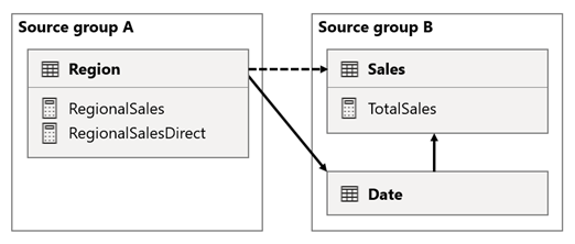
In this scenario, the Region table in source group A has a relationship to the Date table and Sales table in source group B. The relationship between the Region table and the Date table is active, while the relationship between the Region table and the Sales table is inactive. Also, there's an active relationship between the Region table and the Sales table, both of which are in source group B. The Sales table includes a measure named TotalSales, and the Region table includes two measures named RegionalSales and RegionalSalesDirect.
Here are the measure definitions.
TotalSales = SUM(Sales[Sales])
RegionalSales = CALCULATE([TotalSales], USERELATIONSHIP(Region[RegionID], Sales[RegionID]))
RegionalSalesDirect = CALCULATE(SUM(Sales[Sales]), USERELATIONSHIP(Region[RegionID], Sales[RegionID]))
Notice how the RegionalSales measure refers to the TotalSales measure, while the RegionalSalesDirect measure doesn't. Instead, the RegionalSalesDirect measure uses the expression SUM(Sales[Sales]), which is the expression of the TotalSales measure.
The difference in the result is subtle. When Power BI evaluates the RegionalSales measure, it applies the filter from the Region table to both the Sales table and the Date table. Therefore, the filter also propagates from the Date table to the Sales table. In contrast, when Power BI evaluates the RegionalSalesDirect measure, it only propagates the filter from the Region table to the Sales table. The results returned by RegionalSales measure and the RegionalSalesDirect measure could differ, even though the expressions are semantically equivalent.
Important
Whenever you use the CALCULATE function with an expression that's a measure in a remote source group, test the calculation results thoroughly.
Cross source group relationship scenario 2
Consider a scenario when a cross source group relationship has high-cardinality relationship columns.
In this scenario, the Date table is related to the Sales table on the DateKey columns. The data type of the DateKey columns is integer, storing whole numbers that use the yyyymmdd format. The tables belong to different source groups. Further, it's a high-cardinality relationship because the earliest date in the Date table is January 1, 1900 and the latest date is December 31, 2100—so there's a total of 73,414 rows in the table (one row for each date in the 1900-2100 time span).
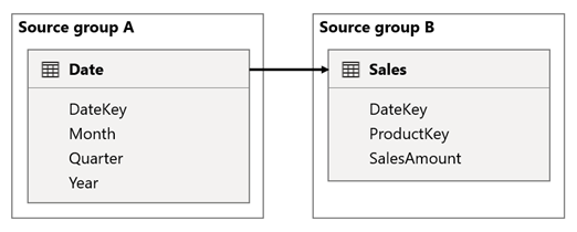
There are two cases for concern.
First, when you use the Date table columns as filters, filter propagation will filter the DateKey column of the Sales table to evaluate measures. When filtering by a single year, like 2022, the DAX query will include a filter expression like Sales[DateKey] IN { 20220101, 20220102, …20221231 }. The text size of the query can grow to become extremely large when the number of values in the filter expression is large, or when the filter values are long strings. It's expensive for Power BI to generate the long query and for the data source to run the query.
Second, when you use Date table columns—like Year, Quarter, or Month—as grouping columns, it results in filters that include all unique combinations of year, quarter, or month, and the DateKey column values. The string size of the query, which contains filters on the grouping columns and the relationship column, can become extremely large. That's especially true when the number of grouping columns and/or the cardinality of the join column (the DateKey column) is large.
To address any performance issues, you can:
- Add the
Datetable to the data source, resulting in a single source group model (meaning, it's no longer a composite model). - Raise the granularity of the relationship. For instance, you could add a
MonthKeycolumn to both tables and create the relationship on those columns. However, by raising the granularity of the relationship, you lose the ability to report on daily sales activity (unless you use theDateKeycolumn from theSalestable).
Cross source group relationship scenario 3
Consider a scenario when there aren't matching values between tables in a cross source group relationship.
In this scenario, the Date table in source group B has a relationship to the Sales table in that source group, and also to the Target table in source group A. All relationships are one-to-many from the Date table relating the Year columns. The Sales table includes a SalesAmount column that stores sales amounts, while the Target table includes a TargetAmount column that stores target amounts.
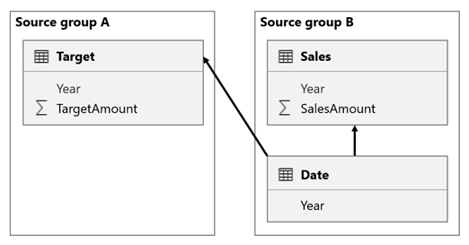
The Date table stores the years 2021 and 2022. The Sales table stores sales amounts for years 2021 (100) and 2022 (200), while the Target table stores target amounts for 2021 (100), 2022 (200), and 2023 (300)—a future year.

When a Power BI table visual queries the composite model by grouping on the Year column from the Date table and summing the SalesAmount and TargetAmount columns, it won't show a target amount for 2023. That's because the cross source group relationship is a limited relationship, and so it uses INNER JOIN semantics, which eliminate rows where there's no matching value on both sides. It will, however, produce a correct target amount total (600), because a Date table filter doesn't apply to its evaluation.
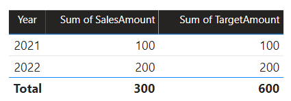
If the relationship between the Date table and the Target table is an intra source group relationship (assuming the Target table belonged to source group B), the visual will include a (Blank) year to show the 2023 (and any other unmatched years) target amount.
Important
To avoid misreporting, ensure that there are matching values in the relationship columns when dimension and fact tables reside in different source groups.
For more information about limited relationships, see Relationship evaluation.
Calculations
You should consider specific limitations when adding calculated columns and calculation groups to a composite model.
Calculated columns
Calculated columns added to a DirectQuery table that source their data from a relational database, like Microsoft SQL Server, are limited to expressions that operate on a single row at a time. These expressions can't use DAX iterator functions, like SUMX, or filter context modification functions, like CALCULATE.
Note
It's not possible to add calculated columns or calculated tables that depend on chained tabular models.
A calculated column expression on a remote DirectQuery table is limited to intra-row evaluation only. However, you can author such an expression, but it will result in an error when it's used in a visual. For example, if you add a calculated column to a remote DirectQuery table named DimProduct by using the expression [Product Sales] / SUM (DimProduct[ProductSales]), you'll be able to successfully save the expression in the model. However, it will result in an error when it's used in a visual because it violates the intra-row evaluation restriction.
In contrast, calculated columns added to a remote DirectQuery table that's a tabular model, which is either a Power BI semantic model or Analysis Services model, are more flexible. In this case, all DAX functions are allowed because the expression will be evaluated within the source tabular model.
Many expressions require Power BI to materialize the calculated column before using it as a group or filter, or aggregating it. When a calculated column is materialized over a large table, it can be costly in terms of CPU and memory, depending on the cardinality of the columns that the calculated column depends on. In this case, we recommend that you add those calculated columns to the source model.
Note
When you add calculated columns to a composite model, be sure to test all model calculations. Upstream calculations may not work correctly because they didn't consider their influence on the filter context.
Calculation groups
If calculation groups exist in a source group that connects to a Power BI semantic model or an Analysis Services model, Power BI could return unexpected results. For more information, see Calculation groups, query and measure evaluation.
Model design
You should always optimize a Power BI model by adopting a star schema design.
Tip
For more information, see Understand star schema and the importance for Power BI.
Be sure to create dimension tables that are separate from fact tables so that Power BI can interpret joins correctly and produce efficient query plans. While this guidance is true for any Power BI model, it's especially true for models that you recognize will become a source group of a composite model. It will allow for simpler and more efficient integration of other tables in downstream models.
Whenever possible, avoid having dimension tables in one source group that relate to a fact table in a different source group. That's because it's better to have intra source group relationships than cross source group relationships, especially for high-cardinality relationship columns. As described earlier, cross source group relationships rely on having matching values in the relationship columns, otherwise unexpected results may be shown in report visuals.
Row-level security
If your model includes user-defined aggregations, calculated columns on import tables, or calculated tables, ensure that any row-level security (RLS) is set up correctly and tested.
If the composite model connects to other tabular models, RLS rules are only applied on the source group (local model) where they're defined. They won't be applied to other source groups (remote models). Also, you can't define RLS rules on a table from another source group nor can you define RLS rules on a local table that has a relationship to another source group.
Report design
In some situations, you can improve the performance of a composite model by designing an optimized report layout.
Single source group visuals
Whenever possible, create visuals that use fields from a single source group. That's because queries generated by visuals will perform better when the result is retrieved from a single source group. Consider creating two visuals positioned side by side that retrieve data from two different source groups.
Use sync slicers
In some situations, you can set up sync slicers to avoid creating a cross source group relationship in your model. It can allow you to combine source groups visually that can perform better.
Consider a scenario when your model has two source groups. Each source group has a product dimension table used to filter reseller and internet sales.
In this scenario, source group A contains the Product table that's related to the ResellerSales table. Source group B contains the Product2 table that's related to the InternetSales table. There aren't any cross source group relationships.
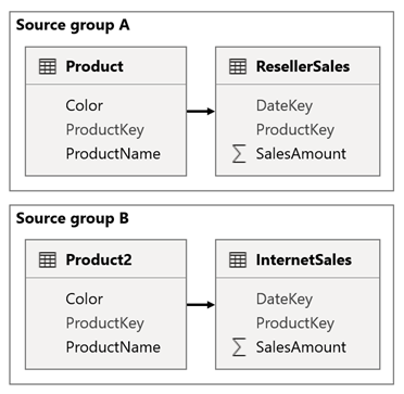
In the report, you add a slicer that filters the page by using the Color column of the Product table. By default, the slicer filters the ResellerSales table, but not the InternetSales table. You then add a hidden slicer by using the Color column of the Product2 table. By setting an identical group name (found in the sync slicers Advanced options), filters applied to the visible slicer automatically propagate to the hidden slicer.
Note
While using sync slicers can avoid the need to create a cross source group relationship, it increases the complexity of the model design. Be sure to educate other users on why you designed the model with duplicate dimension tables. Avoid confusion by hiding dimension tables that you don't want other users to use. You can also add description text to the hidden tables to document their purpose.
For more information, see Sync separate slicers.
Other guidance
Here's some other guidance to help you design and maintain composite models.
- Performance and scale: If your reports were previously live connected to a Power BI semantic model or Analysis Services model, the Power BI service could reuse visual caches across reports. After you convert the live connection to create a local DirectQuery model, reports will no longer benefit from those caches. As a result, you might experience slower performance or even refresh failures. Also, the workload for the Power BI service will increase, which might require you to scale up your capacity or distribute the workload across other capacities. For more information about data refresh and caching, see Data refresh in Power BI.
- Renaming: We don't recommend that you rename semantic models used by composite models, or rename their workspaces. That's because composite models connect to Power BI semantic models by using the workspace and semantic model names (and not their internal unique identifiers). Renaming a semantic model or workspace could break the connections used by your composite model.
- Governance: We don't recommend that your single version of the truth model is a composite model. That's because it would be dependent on other data sources or models, which if updated, could result in breaking the composite model. Instead, we recommended that you publish an enterprise semantic model as the single version of truth. Consider this model to be a reliable foundation. Other data modelers can then create composite models that extend the foundation model to create specialized models.
- Data lineage: Use the data lineage and semantic model impact analysis features before publishing composite model changes. These features are available in the Power BI service, and they can help you to understand how semantic models are related and used. It's important to understand that you can't perform impact analysis on external semantic models that are displayed in lineage view but are in fact located in another workspace. To perform impact analysis on an external semantic model, you need to navigate to the source workspace.
- Schema updates: You should refresh your composite model in Power BI Desktop when schema changes are made to upstream data sources. You'll then need to republish the model to the Power BI service. Be sure to thoroughly test calculations and dependent reports.
Related content
For more information related to this article, check out the following resources.
- Use composite models in Power BI Desktop
- Model relationships in Power BI Desktop
- DirectQuery models in Power BI Desktop
- Use DirectQuery in Power BI Desktop
- Storage mode in Power BI Desktop
- User-defined aggregations
- Questions? Try asking the Fabric Community
- Suggestions? Contribute ideas to improve Fabric