Run hybrid quantum computing jobs with adaptive target profile
Hybrid computing combines classical and quantum computing processes to solve complex problems.
In hybrid computing, the classical code controls the execution of quantum operations based on mid-circuit measurements while the physical qubits remain active. You can use common programming techniques, such as nested conditionals, loops, and function calls, in a single quantum program to run complex problems, reducing the number of shots needed. With qubit reuse techniques, larger programs can run on machines using a smaller number of qubits.
This article explains how to submit hybrid jobs to Azure Quantum using the QIR Adaptive RI target profile. The Adaptive RI target profile offers support for mid-circuit measurements, measurement-based control flow, qubit reset, and classical integer computation.
Prerequisites
- An Azure account with an active subscription. If you don’t have an Azure account, register for free and sign up for a pay-as-you-go subscription.
- An Azure Quantum workspace. For more information, see Create an Azure Quantum workspace.
- If you want to submit Q# standalone programs, you need the following prerequisites:
- Visual Studio Code with the Azure Quantum Development Kit extension installed.
- The latest version of the Azure Quantum Development Kit extension.
- If you wan to submit Python + Q# programs, you need the following prerequisites:
A Python environment with Python and Pip installed.
The Azure Quantum
azure-quantumandqsharppackages.pip install --upgrade azure-quantum qsharp
Supported targets
To run hybrid quantum computing jobs, you need to select a quantum provider that supports the Adaptive RI target profile.
Currently, adaptive target profile in Azure Quantum is supported on Quantinuum targets.
Submitting adaptive RI jobs
To submit hybrid quantum computing jobs, you need to configure the target profile as QIR Adaptive RI, where RI stands for "qubit Reset and Integer computations".
The QIR Adaptive RI target profile offers support for mid-circuit measurements, measurement-based control flow, qubit reset, and classical integer computation.
You can submit hybrid quantum jobs to Azure Quantum as Q# standalone programs or Python + Q# programs. To configure the target profile for hybrid quantum jobs, see the following sections.
To configure the target profile for hybrid jobs in Visual Studio Code, follow these steps:
- Open a Q# program in Visual Studio Code.
- Select View -> Command Palette and type Q#: Set the Azure Quantum QIR target profile. Press Enter.
- Select QIR Adaptive RI.
Once you set QIR Adaptive RI as target profile, you can submit your Q# program as a hybrid quantum job to Quantinuum.
- Select View -> Command Palette and type Q#: Connect to an Azure Quantum workspace. Press Enter.
- Select Azure account, and follow the prompts to connect to your preferred directory, subscription, and workspace.
- Once you are connected, in the Explorer pane, expand Quantum Workspaces.
- Expand your workspace and expand the Quantinuum provider.
- Select any Quantinuum available target, for example quantinuum.sim.h1-1e.
- Select the play icon to the right of the target name to start submitting the current Q# program.
- Add a name to identify the job, and the number of shots.
- Press Enter to submit the job. The job status displays at the bottom of the screen.
- Expand Jobs and hover over your job, which displays the times and status of your job.
Supported features
The following table lists the supported features for hybrid quantum computing with Quantinuum in Azure Quantum.
| Supported feature | Notes |
|---|---|
| Dynamics values | Bools and integers whose value depend on a measurement result |
| Loops | Classically-bounded loops only |
| Arbitrary control flow | Use of if/else branching |
| Mid-circuit measurement | Utilizes classical register resources |
| Qubit reuse | Supported |
| Real-time classical compute | 64-bit signed integer arithmetic Utilizes classical register resources |
The QDK provides target-specific feedback when Q# language features aren't supported for the selected target. If your Q# program contains unsupported features when running hybrid quantum jobs, you'll receive an error message at design-time. For more information, see the QIR wiki page.
Note
You need to select the appropriate QIR Adaptive RI target profile to obtain appropriate feedback when using Q# features that the target doesn't support.
To see the supported features in action, copy the following code into a Q# file and add the subsequent code snippets.
import Microsoft.Quantum.Measurement.*;
import Microsoft.Quantum.Math.*;
import Microsoft.Quantum.Convert.*;

operation Main() : Result {
    use (q0, q1) = (Qubit(), Qubit());
    H(q0);
    let r0 = MResetZ(q0);

    // Copy here the code snippets below to see the supported features
    // in action.
    // Supported features include dynamic values, classically-bounded loops,
    // arbitrary control flow, and mid-circuit measurement.

    r0
}
Quantinuum supports dynamic bools and integers, which means bools and integers that depend on measurement results. Note that r0 is a Result type that can be used to generate dynamic bool and integer values.
        let dynamicBool = r0 != Zero;
        let dynamicBool = ResultAsBool(r0);
        let dynamicInt = dynamicBool ? 0 | 1;
Quantinuum supports dynamic bools and integers, however, it doesn't support dynamic values for other data types, such as double. Copy the following code to see feedback about the limitations of dynamic values.
        let dynamicDouble = r0 == One ? 1. | 0.; // cannot use a dynamic double value
        let dynamicInt = r0 == One ? 1 | 0;
        let dynamicDouble = IntAsDouble(dynamicInt); // cannot use a dynamic double value
        let dynamicRoot = Sqrt(dynamicDouble); // cannot use a dynamic double value
Even though dynamic values are not supported for some data types, those data types can still be used with static values.
    let staticRoot = Sqrt(4.0);
    let staticBigInt = IntAsBigInt(2);
Even dynamic values of supported typed can't be used in certain situations. For example, Quantinuum doesn't support dynamic arrays, that is, arrays whose size depends on a measurement result. Quantinuum doesn't support dynamically-bounded loops either. Copy the following code to see the limitations of dynamic values.
        let dynamicInt = r0 == Zero ? 2 | 4;
        let dynamicallySizedArray = [0, size = dynamicInt]; // cannot use a dynamically-sized array
        let staticallySizedArray = [0, size = 10];
        // Loops with a dynamic condition are not supported by Quantinuum.
        for _ in 0..dynamicInt {
            Rx(PI(), q1);
        }

        // Loops with a static condition are supported.
        let staticInt = 3;
        for _ in 0..staticInt {
            Rx(PI(), q1);
        }
Quantinuum supports control flow, including if/else branching, using both static and dynamic conditions. Branching on dynamic conditions is also known as branching based on measurement results.
        let dynamicInt = r0 == Zero ? 0 | 1;
        if dynamicInt > 0 {
            X(q1);
        }
        let staticInt = 1;
        if staticInt > 5 {
            Y(q1);
        } else {
            Z(q1);
        }
Quantinuum supports loops with classical conditions and including if expressions.
        for idx in 0..3 {
            if idx % 2 == 0 {
                Rx(ArcSin(1.), q0);
                Rz(IntAsDouble(idx) * PI(), q1)
            } else {
                Ry(ArcCos(-1.), q1);
                Rz(IntAsDouble(idx) * PI(), q1)
            }
        }
Quantinuum supports mid-circuit measurement, that is, branching based on measurement results.
        if r0 == One {
            X(q1);
        }
        let r1 = MResetZ(q1);
        if r0 != r1 {
            let angle = PI() + PI() + PI()* Sin(PI()/2.0);
            Rxx(angle, q0, q1);
        } else {
            Rxx(PI() + PI() + 2.0 * PI() * Sin(PI()/2.0), q1, q0);
        }
Estimating the cost of a hybrid quantum computing job
You can estimate the cost of running a hybrid quantum computing job on Quantinuum hardware by running it on an emulator first.
After a successful run on the emulator:
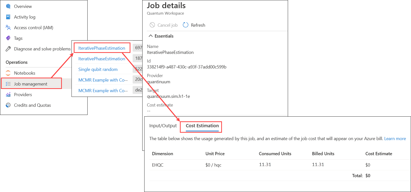
- In your Azure Quantum workspace, select Job management.
- Select the job you submitted.
- In the Job details popup, select Cost Estimation to view how many eHQCs (Quantinuum emulator credits) were used. This number translates directly to the number of HQCs (Quantinuum quantum credits) that are needed to run the job on Quantinuum hardware.
Note
Quantinuum unrolls the entire circuit and calculates the cost on all code paths, whether they're conditionally executed or not.
Hybrid quantum computing samples
The following samples can be found in Q# code samples repository. They demonstrate the current feature set for hybrid quantum computing.
Three-qubit repetition code
This sample demonstrates how to create a three-qubit repetition code that can be used to detect and correct bit flip errors.
It leverages integrated hybrid computing features to count the number of times error correction was performed while the state of a logical qubit register is coherent.
You can find the code sample here.
Iterative phase estimation
This sample program demonstrates an iterative phase estimation within Q#. It uses iterative phase estimation to calculate an inner product between two 2-dimensional vectors encoded on a target qubit and an ancilla qubit. An additional control qubit is also initialized which is the only qubit used for measurement.
The circuit begins by encoding the pair of vectors on the target qubit and the ancilla qubit. It then applies an Oracle operator to the entire register, controlled off the control qubit, which is set up in the $\ket +$ state. The controlled Oracle operator generates a phase on the $\ket 1$ state of the control qubit. This can then be read by applying an H gate to the control qubit to make the phase observable when measuring.
You can find the code sample here.
Note
This sample code was written by members of KPMG Quantum team in Australia and falls under an MIT License. It demonstrates expanded capabilities of QIR Adaptive RI targets and makes use of bounded loops, classical function calls at run time, nested conditional if statements, mid circuit measurements, and qubit reuse.