Inference and evaluation of forecasting models
This article introduces concepts related to model inference and evaluation in forecasting tasks. For instructions and examples for training forecasting models in AutoML, see Set up AutoML to train a time-series forecasting model with SDK and CLI.
After you use AutoML to train and select a best model, the next step is to generate forecasts. Then, if possible, evaluate their accuracy on a test set held out from the training data. To see how to setup and run forecasting model evaluation in automated machine learning, see Orchestrating training, inference, and evaluation.
Inference scenarios
In machine learning, inference is the process of generating model predictions for new data not used in training. There are multiple ways to generate predictions in forecasting due to the time dependence of the data. The simplest scenario is when the inference period immediately follows the training period and you generate predictions out to the forecast horizon. The following diagram illustrates this scenario:
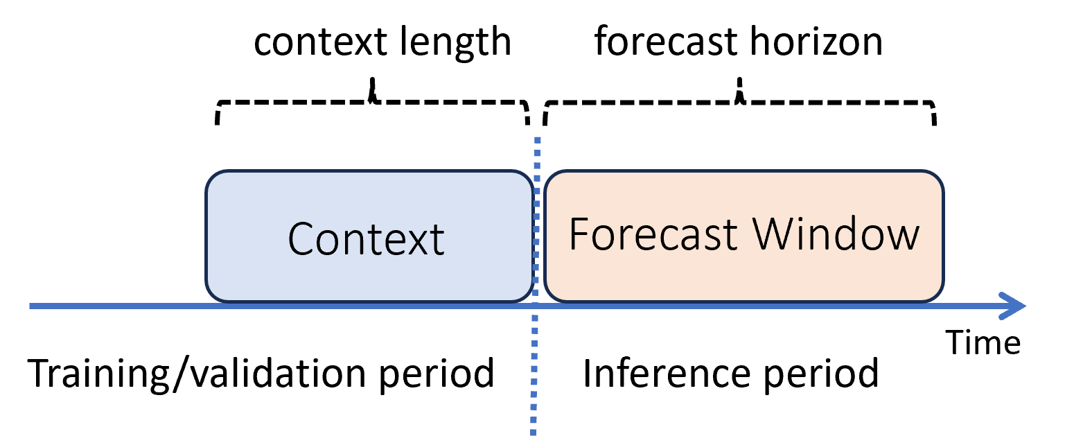
The diagram shows two important inference parameters:
- The context length is the amount of history that the model requires to make a forecast.
- The forecast horizon is how far ahead in time the forecaster is trained to predict.
Forecasting models usually use some historical information, the context, to make predictions ahead in time up to the forecast horizon. When the context is part of the training data, AutoML saves what it needs to make forecasts. There's no need to explicitly provide it.
There are two other inference scenarios that are more complicated:
- Generating predictions farther into the future than the forecast horizon
- Getting predictions when there's a gap between the training and inference periods
The following subsections review these cases.
Predict past the forecast horizon: recursive forecasting
When you need forecasts past the horizon, AutoML applies the model recursively over the inference period. Predictions from the model are fed back as input to generate predictions for subsequent forecasting windows. The following diagram shows a simple example:
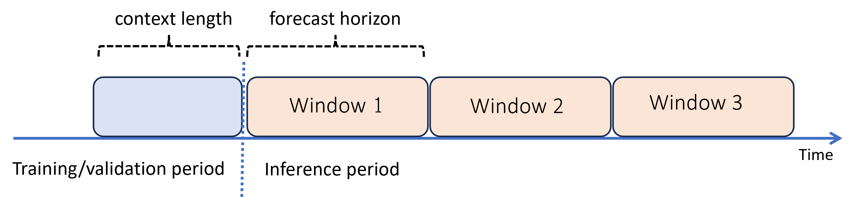
Here, machine learning generates forecasts on a period three times the length of the horizon. It uses predictions from one window as the context for the next window.
Warning
Recursive forecasting compounds modeling errors. Predictions become less accurate the farther they are from the original forecast horizon. You might find a more accurate model by re-training with a longer horizon.
Predict with a gap between training and inference periods
Suppose that after you train a model, you want to use it to make predictions from new observations that weren't yet available during training. In this case, there's a time gap between the training and inference periods:
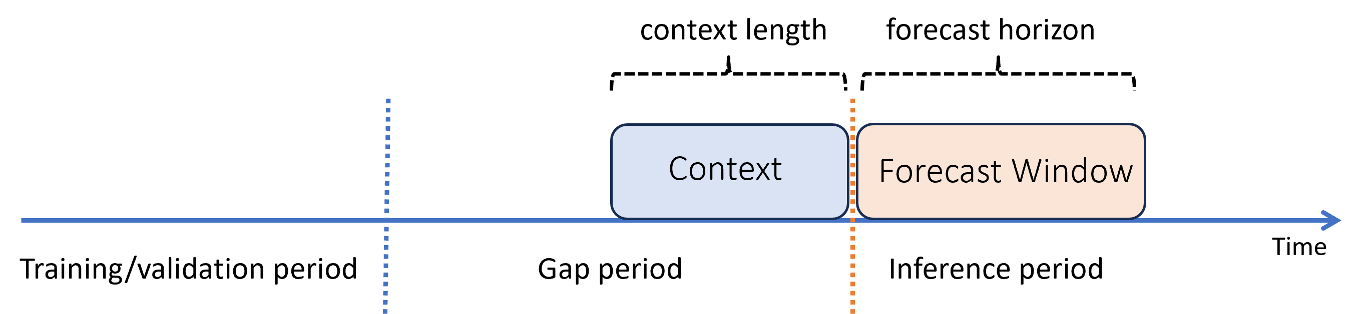
AutoML supports this inference scenario, but you need to provide the context data in the gap period, as shown in the diagram. The prediction data passed to the inference component needs values for features and observed target values in the gap and missing values or NaN values for the target in the inference period. The following table shows an example of this pattern:
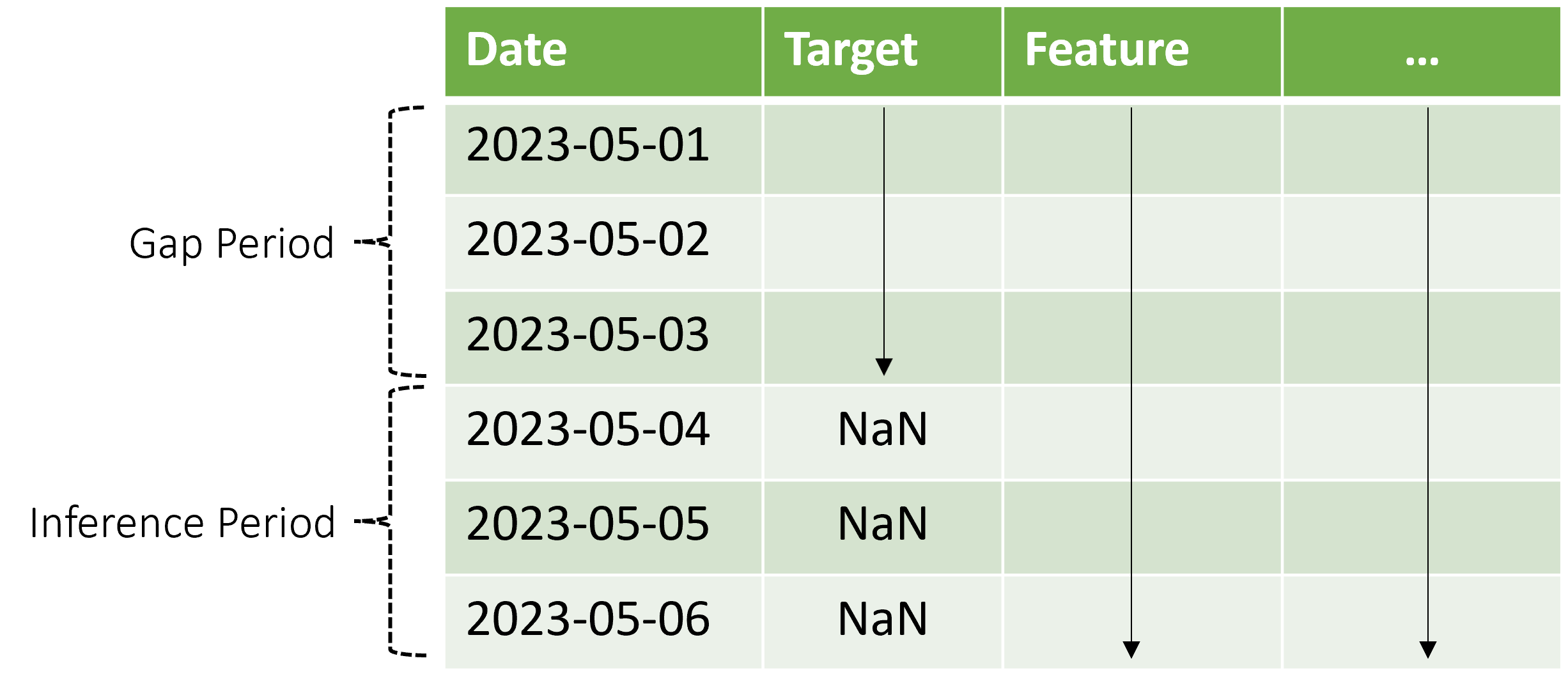
Known values of the target and features are provided for 2023-05-01 through 2023-05-03. Missing target values starting at 2023-05-04 indicate that the inference period starts at that date.
AutoML uses the new context data to update lag and other lookback features, and also to update models like ARIMA that keep an internal state. This operation doesn't update or refit model parameters.
Model evaluation
Evaluation is the process of generating predictions on a test set held-out from the training data and computing metrics from these predictions that guide model deployment decisions. Accordingly, there's an inference mode suited for model evaluation: a rolling forecast.
A best practice procedure for evaluating a forecasting model is to roll the trained forecaster forward in time over the test set, averaging error metrics over several prediction windows. This procedure is sometimes called a backtest. Ideally, the test set for the evaluation is long relative to the model's forecast horizon. Estimates of forecasting error might otherwise be statistically noisy and, therefore, less reliable.
The following diagram shows a simple example with three forecasting windows:
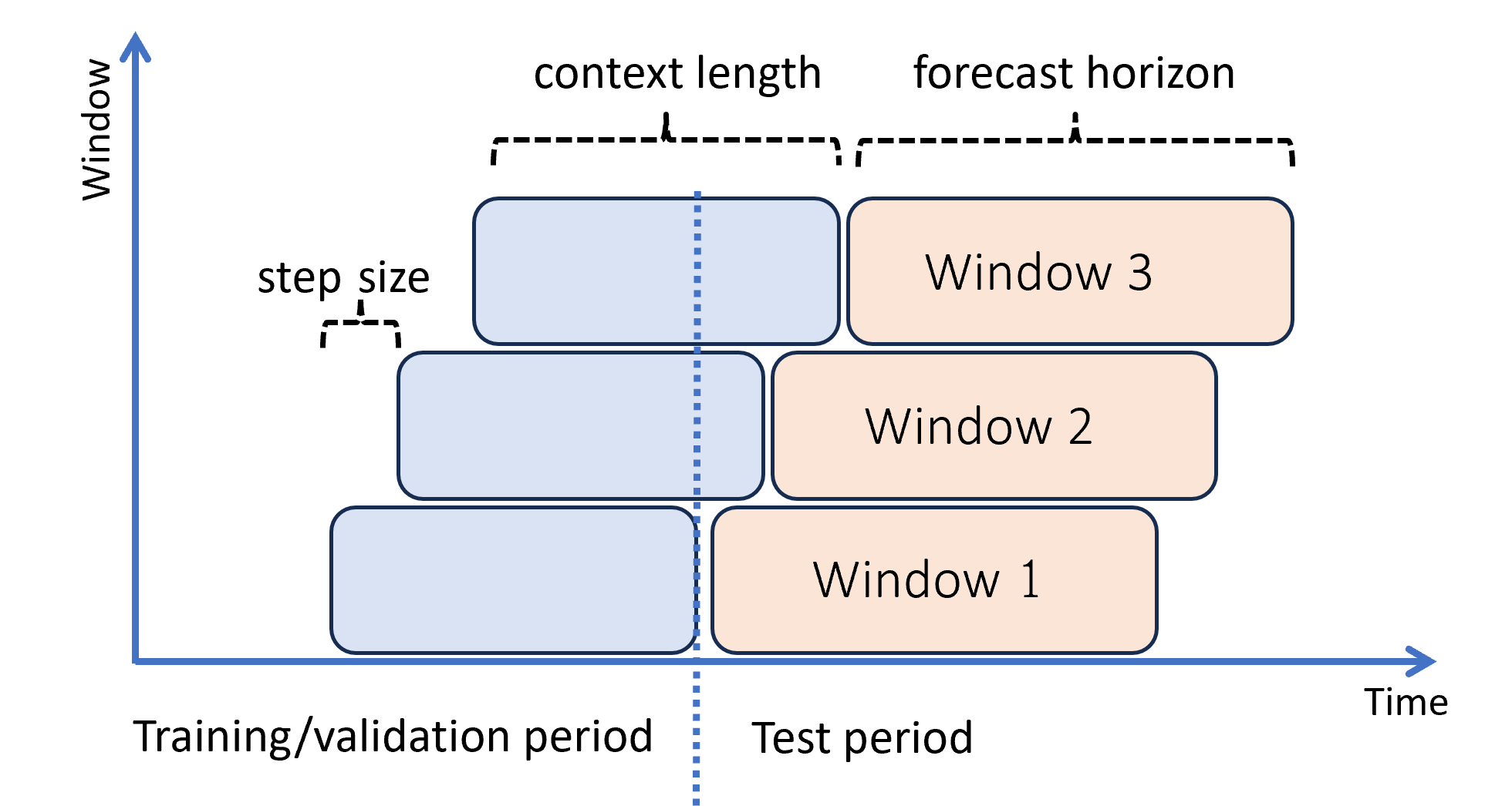
The diagram illustrates three rolling evaluation parameters:
- The context length is the amount of history that the model requires to make a forecast.
- The forecast horizon is how far ahead in time the forecaster is trained to predict.
- The step size is how far ahead in time the rolling window advances on each iteration on the test set.
The context advances along with the forecasting window. Actual values from the test set are used to make forecasts when they fall within the current context window. The latest date of actual values used for a given forecast window is called the origin time of the window. The following table shows an example output from the three-window rolling forecast with a horizon of three days and a step size of one day:
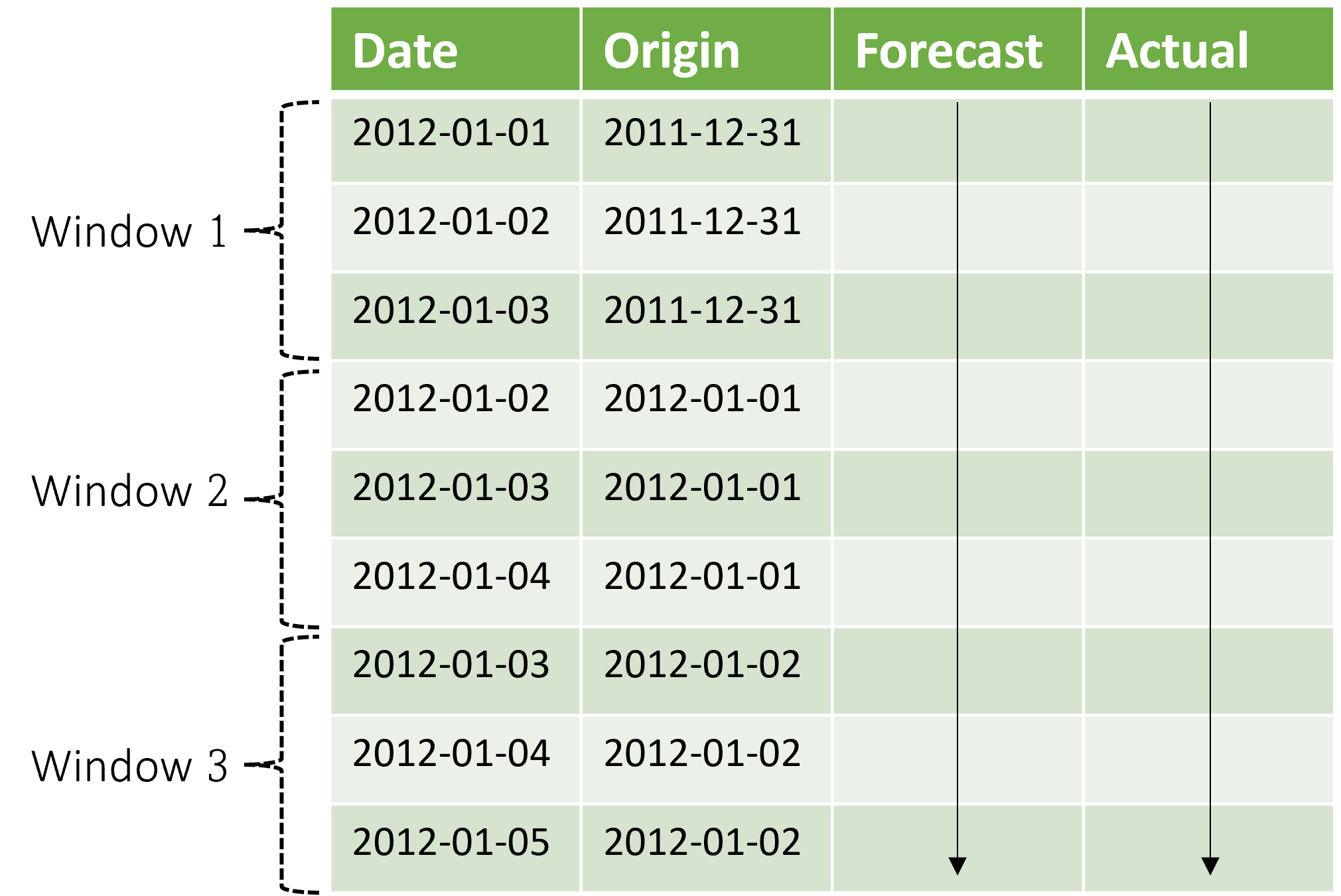
With a table like this, you can visualize the forecasts versus the actuals and compute desired evaluation metrics. AutoML pipelines can generate rolling forecasts on a test set with an inference component.
Note
When the test period is the same length as the forecast horizon, a rolling forecast gives a single window of forecasts up to the horizon.
Evaluation metrics
The specific business scenario usually drives the choice of evaluation summary or metric. Some common choices include the following examples:
- Plots of observed target values versus forecasted values to check that certain dynamics of the data that the model captures
- Mean absolute percentage error (MAPE) between actual and forecasted values
- Root mean squared error (RMSE), possibly with a normalization, between actual and forecasted values
- Mean absolute error (MAE), possibly with a normalization, between actual and forecasted values
There are many other possibilities, depending on the business scenario. You might need to create your own post-processing utilities for computing evaluation metrics from inference results or rolling forecasts. For more information on metrics, see Regression/forecasting metrics.
Related content
- Learn more about how to set up AutoML to train a time-series forecasting model.
- Learn about how AutoML uses machine learning to build forecasting models.
- Read answers to frequently asked questions about forecasting in AutoML.