C#: Multitasking Case Study - Quadratic Sieve
Microsoft C# .NET Framework 4.5.2 has two excellent means of adding parallel processing to an application, namely, multitasking and parallel loops. In this case study we concentrate on multitasking.
All experiments mentioned in this article were run on a relatively new (late October 2015) Dell XPS 8900 computer with an Intel Core i7-6700K CPU operating at a clock frequency of 4.00 GHz with 16 GB DDR4 memory and a 2 TB hard-drive with a 32 GB SSD buffer. The code was compiled and run in Debug mode within the Visual Studio 2015 Community version.
The quadratic sieve is a means of factoring relatively large integers. Although the algorithm has been largely supplanted by the multiple polynomial quadratic sieve and the special and general number field sieve, it is still an interesting and useful introduction to modern factoring methods from a pedagogical point of view. The algorithm has four computationally intense phases:
Creation of the prime factor base consisting of t factors
Finding smooth numbers using the polynomial q(x) = (x + m)^2 - n, where m = Sqrt(n), and n is the number to be factored, we need t1 = t + 1 of these numbers
Finding the kernel of the exponent matrix (modulo 2) found in step 2
Finding the factors of the original number using the vectors of step 3 and numbers of step 2
Steps 2 and 4 dominate the runtime of the whole application. Therefore, these are the two parts of the algorithm that could benefit from parallel processing. The sequential version of this pair of test programs uses 3.21 Algorithm Quadratic sieve algorithm for factoring integers from Handbook of Applied Cryptography by Alfred J. Menezes, Paul C. van Oorschot, and Scott A. Vanstone.
For phase 4 of the applications we use Algorithm 2.3.1 (Kernel of a Matrix) found in A Course in Computational Algebraic Number Theory by Henri Cohen. We tried in vain to speed up this algorithm by the introduction of two parallel loops. Adding a parallel loop to the vector initialization loop did not statistically improve the algorithm's runtime. The addition of a second parallel loop actually slowed down the code so we abandoned attempts to rev up this important phase.
Now onto phase 2. The code for this phase in the sequential variant is illustrated next:
for (int i = 1; i <= maxI; i++)
{
 if (i == 1)
 {
 x = 0;
 }

 else if  (i % 2 == 0)
 {
 x = +i / 2;
 }

 else
 {
 x = -i / 2;
 }

 BigInteger xm = x + m, b = xm * xm - n;
 List<PrimeExpon> lpe = new  List<PrimeExpon>();

 if (TrialDivision(b, p, lpe))
 {
 for (int j = 0; j < t; j++)
 e[count, j] = v[count, j] = 0;

 for (int j = 0; j < t; j++)
 {
 long q = p[j];

 for (int k = 0; k < lpe.Count; k++)
 {
 PrimeExpon pe = lpe[k];

 if (q == pe.prime)
 {
 e[count, j] = (sbyte)pe.expon;
 v[count, j] = (sbyte)(pe.expon % 2);
 break;
 }
 }
 }

 ai.Add(xm);
 bi.Add(b);

 count++;
Since the test-bed CPU has four cores and eight logical processors we transform the preceding code into four concurrent tasks. First we define the Action's state object.
public struct  State
{
 public int  i0, i1, number;
 public BigInteger m, n;
 public List<int> p;
 public List<BigInteger> la, lb;
 public List<List<PrimeExpon>> lpel;

 public State(
 int i0, int i1, int number,
 BigInteger m, BigInteger n,
 List<int> p)
 {
 this.i0 = i0;
 this.i1 = i1;
 this.number = number;
 this.m = m;
 this.n = n;
 this.p = p;
 la = new  List<BigInteger>();
 lb =  new  List<BigInteger>();
 lpel = new  List<List<PrimeExpon>>();
 }
}
Next we introduce the Action that carries out both a loop and the trial division method of the sequential version:
public void  FactorTask(object o)
{
 int num = 0;
 BigInteger x = 0;
 HCSRAlgorithm hc = new  HCSRAlgorithm(1);
 State s = (State)o;

 for (int i = s.i0; i <= s.i1; i++)
 {
 if (i == 1)
 {
 x = 0;
 }

 else if  (i % 2 == 0)
 {
 x = +i / 2;
 }

 else
 {
 x = -i / 2;
 }

 BigInteger xm = x + s.m, b = xm * xm - s.n;
 List<PrimeExpon> lpe = new  List<PrimeExpon>();
 int result = -1;
 BigInteger tb = b, tsb;
 PrimeExpon pe = new  PrimeExpon();

 if (b == 0 || b == 1 || b == -1)
 result = -1;

 else
 {
 if (tb < 0)
 {
 tb = -tb;
 pe.prime = -1;
 pe.expon = +1;
 lpe.Add(pe);
 }

 tsb = Sqrt(tb);

 for (int j = 1; result == -1 && j < s.p.Count; j++)
 {
 int exp = 0;
 BigInteger q = s.p[j];

 if (q > tsb)
 {
 result = 0;
 }

 else if  (tb % q == 0)
 {
 do
 {
 exp++;
 tb /= q;
 } while  (tb % q == 0);

 pe.prime = (int)q;
 pe.expon = exp;
 lpe.Add(pe);

 if (tb == 1 || !hc.Composite(tb, 20))
 {
 result = 1;
 }
 }
 }
 }

 if (result == 1)
 {
 s.la.Add(xm);
 s.lb.Add(b);
 s.lpel.Add(lpe);
 num++;

 if (num == s.number)
 {
 return;
 }
 }
 }
}
The final step is to initialize the four tasks state objects and to launch the tasks to concurrently carry out phase 2 of the algorithm:
BigInteger m = Sqrt(n), x = 0;

states[0] =  new  State(  1, 10000000, number, m, n, p);
states[1] =  new  State(10000001, 20000000, number, m, n, p);
states[2] =  new  State(20000001, 30000000, number, m, n, p);
states[3] =  new  State(30000001, 40000000, number, m, n, p);
sw.Restart();

for (int j = 0; j < 4; j++)
{
 tasks[j] = new  Task(FactorTask, states[j]);
 tasks[j].Start();
}

Task.WaitAll(tasks);

// merge data from the four tasks

for (int j = 0; count < t1 && j < 4; j++)
{
 State s = states[j];

 if (s.la.Count != number)
 return -1;

 for (int k = 0; count < t1 && k < s.number; k++)
 {
 la.Add(s.la[k]);
 lb.Add(s.lb[k]);

 for (int l = 0; l < t; l++)
 e[count, l] = v[count, l] = 0;

 List<PrimeExpon> lpe = s.lpel[k];

 for (int l = 0; l < t; l++)
 {
 int q = s.p[l];

 for (int u = 0; u < lpe.Count; u++)
 {
 PrimeExpon pe = lpe[u];

 if (q == pe.prime)
 {
 e[count, l] = (sbyte)pe.expon;
 v[count, l] = (sbyte)(pe.expon % 2);
 break;
 }
 }
 }

 count++;
 }
}

sw.Stop();
times.Add(sw.ElapsedMilliseconds);
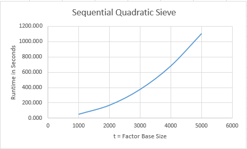
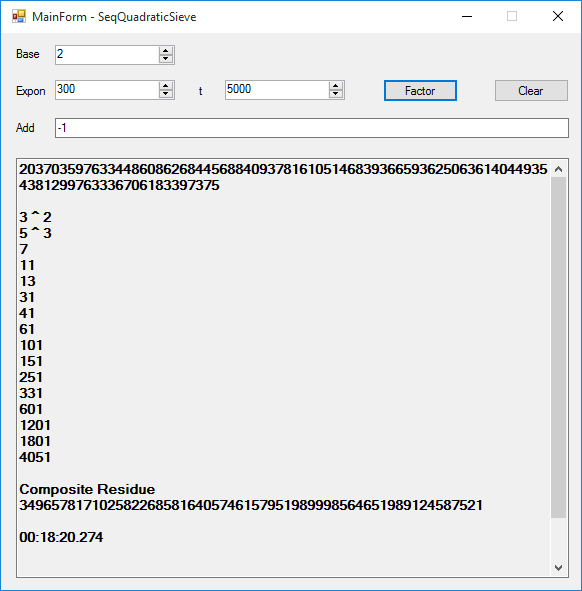
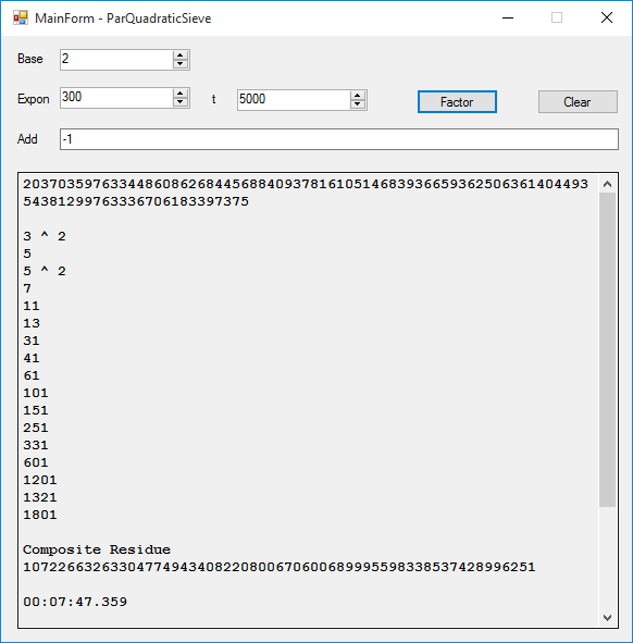
The results are pretty astonishing. The parallel also known as multitasking version dramatically cuts down the runtime of the factoring of our test case number. We attempt to completely factor the large Mersenne number, M(300) = 2 ^ 300 - 1. We chose this number since it is rich in a factors less than 1000000. These factors are: 3^2, 5^3, 7, 11, 13, 31, 41, 61, 101, 151, 251, 331, 601, 1201, 1321, 1801, 4051, 8101, 63901, 100801, and 268501. Two additional factors are: 10567201, 13334701, and a 22 decimal digit composite number. Below is a table of runtimes in seconds for the sequential variant varying t = the number of prime numbers in the factor base:
| t | Time (s) | Factors Found |
| 1000 | 51.898 | 11 |
| 2000 | 169.596 | 15 |
| 3000 | 375.588 | 14 |
| 4000 | 680.609 | 13 |
| 5000 | 1100.274 | 16 |
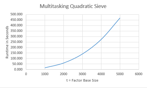
Now we show the multitasking program's analogous results:
| t | Time (s) | Factors Found |
| 1000 | 17.277 | 12 |
| 2000 | 60.537 | 14 |
| 3000 | 142.134 | 15 |
| 4000 | 273.330 | 14 |
| 5000 | 467.359 | 16 |
Graphs of the preceding table data are displayed below:
The phases required the runtimes in milliseconds are shown in the table below for the parallel version:
| t | Phase 1 | Phase 2 | Phase 3 | Phase 4 |
| 1000 | 22 | 14988 | 2245 | 15 |
| 2000 | 76 | 42761 | 17659 | 20 |
| 3000 | 69 | 85091 | 56942 | 29 |
| 4000 | 110 | 140494 | 132671 | 42 |
| 5000 | 122 | 212010 | 255138 | 57 |
In conclusion we see that studying an application using the Stopwatch object of the Diagnostics facility that a software engineer and/or programmer can easily see what parts of an application need optimization. A judicious usage of parallel loops and/or concurrent tasks can dramatically change the runtime performance of an executable.


