Visual Basic: Genetic algorithm to solve 2D Mazes
Scope
In this article, as a sequel to Genetic algorithm for icon generation in Visual Basic, we'll see how genetic algorithms can be applied to solve problems. The approach is particularly suited to a requirement where we don't have a prior model (or, an ideal target to reach), but know the optimal parameters which tend to a solution. In other words, we'll discuss genetic algorithms (GA) in the solutions optimization context. The language in which we'll develop a sample application will be Visual Basic .NET again.
Introduction
In the last article we considered how, starting from a given graphical model, it's possible to generate a set of random and chaotic solutions which will evolve towards our target through the constant selection of the best samples from each set, crossing their information to create new champions, perhaps ameliorative. Though those are interesting ways to explore GAs, when we discuss those coded to grow towards a strict model have the obvious need of a starting complete and ideal solution. That means if we don't have a final result to match each solution we create, we won't have any mean to evolve beyond chaos, closing our algorithm in an infinite loop of random samples, because they won't be oriented to any specificity.
Obviously, a GA must always have a target, in a way or another. However, a monolithic model isn't always necessary, but - after we have defined the optimal conditions we expect - let the algorithm find solutions that meet those requirements (or, the optimal solution to a given problem). There are lot of practical applications for that, regarding many fields of human knowledge. But since we learn better when we play with something, we'll see here an example of a Visual Basic GA oriented to solve a 2D maze, trying - through previously saw functionalities - not only to join two points in space, but to do it in one of the better ways - i.e. searching for the shorter path.
A brief recap
Let's review the main concepts to refresh your memory.
A GA is so named because it tries to mime those biological processes at the core of species evolution. We could say it aims at creating a computer model able to auto-tune itself to a specific context, generating individuals (solutions to a given problem) which will be used to evaluate a the real achieving of a given objective. The problem to be solved is the digital equivalent of the biological context in which individuals move, obeying the "fittest's survive" tenet. In the previous article i've used the example of a world filled with predators, in which the fastest inhabitants (more apt to an efficient flight) or the more pugnacious (mode apt to an efficient fight) represents the best candidates to survive, if compared with slower o weaker samples. In the same way, if we have a digital target (equivalent of the base parameter of biological survival), we could tell about "apt individuals" in the measure in which potential solutions get nearer to the given objective. Among them, in the same way nature does, we'll try to identify the best solutions to get them reproduce, generating new solutions that will bear their parents peculiarities. A quick sample about it has been shown in the first article: given a certain graphical icon (an array of bytes which produces an image), starting from a fixed number of chaotic solutions, in each generations the best solutions are those akin to the model at which they aim.
The biological inspiration of GA passes through its terminology, too. In it, we'll speak of:
- The concept of individual/chromosome, of a single solution to a given problem;
- Population, or the whole set of possible solutions;
- Gene, or a parte (byte) of an individual;
- Fitness, to be intended as the rate of validity in a solution/individual;
- Crossing-over, or the solutions recombination to produce new models, new chromosomes/individuals;
- Mutation, to be intended as random changes (or pseudo-random) which can occur inside a solution;
All those concepts are valid in a digital world, and must be implemented in some way to speak bout a real GA-based solution, or a solution which can autoevolve. The developer must define each one of them, in theoretical and practical means to deal with each phase.
Optimizing a solution
In principle, when dealing with the case of image replication too, when taling about GAs we could always think about optimization. In facts, each GA case is - ultimately - the search for the best solution, whenever it refers to reach the ideal target or falling in a satisfying local optimum. With the term "local optimum", we indicate the inability to progress further a giver precision rate, due to certain population characteristics which, after recombination, doesn't produce improvements. A method to prevent stagnation is possibly applied through mutation, through which we introduce - on a random basis - changes in the newly created solutions, to maintain a little constant of chaos in transmitting information from a generation to the next one.
Despite we could always refer to the concept of optimization, it becomes more evident when applied to a logistical problem. Let's suppose we are inside a maze, which provides several ways to reach the destination. In it we could move as the internal topography allows, and its not to be excluded we could go back on our steps, or never reach destination. Essentially, in such a labyrinth there are many ways to reach a solution...but a solution which will be better compared to others exists, too. In such a place, the best road is the one which leads us from start point to end in a straight way, in the least steps possible (i.e., the optimal solution). A GA could help us to spot that path, without previously knowing what the possibilities are. We note it isn't just about finding a way to arrive, but to test its validity, considering what will be better.
Base structure
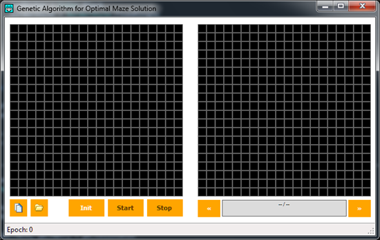
To be able to think about a labyrinth, we must have a labyrinth. Here we'll see the basis i've used in my example, to briefly explain what will be the ground on which we will work. As usual, at the end of the article you'll find a link to download the source code of the example, which i invite you to consult for a detailed view about those aspects that won't be treated in the present lines. Running the sample code, we'll see a window like this:
The program will create two windows with 20 cells per side, which will be used as a graphical representation on the elements constituting the user-defined labyrinth (on the left) and the one which will show the found solutions (on the right). In the left panel, the user can click each cell a given number of times. Follows a short table to explain what each click will produce on a cell:
- 1 Click = "Wall" cell (gray, it wil be impassable)
- 2 Click = Start point (green, the entering point of the labyrinth)
- 3 Click = End point (red, the exit point of the labyrinth)
- 4 Click = Valid cell (not used in labyrinth creating, it will belong to the GA)
- 5 Click = "Free" cell (black, a cell that can be crossed)
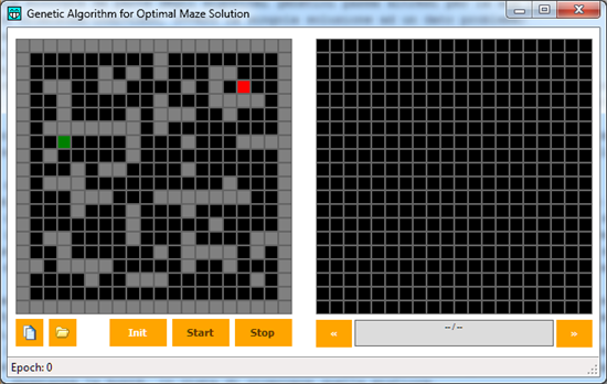
To be able to test the program in a quick way, i've implemented two buttons to save and load previously created labyrinths. In the source code's package, i've made available the "test_maze.txt" file, which is the one we use in this example. Loading that file, we'll obtain the following labyrinth:
We can immediately see there are many possible solutions between start and end point. Before getting into the GA part, i will spend somw words about the creation of the labyrinth, to explain its underlying logics: it will be useful for a better understanding of the algorithm itself.
Implementing a labyrinth in VB
Our labyrinth has a base made by a bidimensional byte array, named sourceMaze(). Each cell of it represents an array position, in its form (X,Y). Each of those bytes is set to a value which represents the current state of a particular cell. Those values are associated with an enumeration, visible in the Globals.vb file:
Module Globals
    Public Const  MAZESIZE As  Byte = 20
    Public Const  MAZESIDE As  Byte = 15

    Public Enum  CELLSTATE
        Free = 0
        Wall = 1
        Start = 2
        Finish = 3
        Valid = 4
        FakeWall = 5
    End Enum
End Module
There is an additional value compared to the values discussed above, namely FakeWall = 5. We will talk about it soon, when we'll analyze how the solutions are created.
During the Form load, a call to the routine which draws the labyrinths is made. Drawing operations are done through MazeCell controls, which are PictureBox extensions created to contain data from the data array
Private Sub  GenerateMaze(container As Panel)
    Dim _TOP As Integer  = 0
    Dim _LEFT As Integer  = 0

    For _Y As Integer  = 0 To  MAZESIZE - 1
        For _X As Integer  = 0 To  MAZESIZE - 1

            Dim pb As New  MazeCell
            With pb
                .Name = container.Name & _Y.ToString("00") & _X.ToString("00")
                .Top = _TOP
                .Left = _LEFT
                .Width = MAZESIDE
                .Height = MAZESIDE
                .BackColor = Color.Black
                .BorderStyle = BorderStyle.FixedSingle
                .Cursor = Cursors.Hand

                .MatX = _X
                .MatY = _Y

                AddHandler pb.Click, AddressOf MazeClickCell
            End With

            _LEFT += MAZESIDE
            container.Controls.Add(pb)
        Next
        _LEFT = 0
        _TOP += MAZESIDE
    Next
End Sub
GenerateMaze() needs an argument of type Panel, which represents the owner control in which we'll generate our strcture. Next, with two nested loops, cells are created. They will be bound with the sourceMaze array during MazeClickCell event, defined as:
Private Sub  MazeClickCell(sender As Object, e As  EventArgs)
    Dim pb As MazeCell = CType(sender, MazeCell)

    pb.CellStatus += 1
    If pb.CellStatus > CELLSTATE.Valid Then pb.CellStatus = CELLSTATE.Free

    sourceMaze(pb.MatX, pb.MatY) = pb.CellStatus
    pb.BackColor = pb.CellBrush
End Sub
We can note MazeCell controls, in comparison with standard PictureBox, have additional properties, like MatX, which identifies cell's abscissa in the matrix, MatY, which represents ordinate, CellStatus, which exposes a cell's content, and CellBrush, which - following the status of a cell - represents the cell itself with a color. The source code which realizes the MazeCell extension is the following:
Public Class  MazeCell
    Inherits PictureBox

    Dim _STATUS As Byte  = 0
    Dim _MATX As Byte  = 0
    Dim _MATY As Byte  = 0

    Public Property  CellStatus As  Byte
        Get
            Return _STATUS
        End Get
        Set(value As  Byte)
            _STATUS = value
        End Set
    End Property

    Public ReadOnly  Property CellBrush As Color
        Get
            Select Case  CellStatus
                Case CELLSTATE.Free
                    Return Color.Black
                Case CELLSTATE.Valid
                    Return Color.Violet
                Case CELLSTATE.Start
                    Return Color.Green
                Case CELLSTATE.Finish
                    Return Color.Red
                Case CELLSTATE.Wall
                    Return Color.Gray
                Case CELLSTATE.FakeWall
                    Return Color.Yellow
            End Select
        End Get
    End Property

    Public Property  MatX As  Byte
        Get
            Return _MATX
        End Get
        Set(value As  Byte)
            _MATX = value
        End Set
    End Property

    Public Property  MatY As  Byte
        Get
            Return _MATY
        End Get
        Set(value As  Byte)
            _MATY = value
        End Set
    End Property

    Public ReadOnly  Property StringMatrix As String
        Get
            Return _MATX.ToString & ";" & _MATY.ToString
        End Get
    End Property
End Class
The present structure allows the user to define his own base labyrinth, to be then passed as a base for the GA, or saving it for future reference (i've implemented - but not optimized - basic routines to save and load labyrinth data, but i won't discuss them here, to focus on the topic's fundamentals).
Genetic algorithm logics
Now that we have an operative context, we can start reasoning about the explorative possibilities of an automaton. We've mentioned above about the rules to be applied for each type of cell, and consequently we know what are the basic requisites a generic explorative algorithm must possess (please note: generic, not genetic). We know it must start moving from the green cell, trying to reach the red one, without crossing grey ones. All the black cells can be explored/stepped over. We can think about a routine wich, given a start point, evaluate the status of the four adjacent cells, to recursively cross those which will be considered free.
In other words, being solverBytes() the array containing a given solution, a function like this will do:
Private Function  Solve(_X As  Integer, _Y As Integer) As  Boolean
    If solverBytes(_endPos(0), _endPos(1)) = CELLSTATE.Valid  Then  Return True

    If solverBytes(_X + 1, _Y) = CELLSTATE.Free Or solverBytes(_X + 1, _Y) = CELLSTATE.Start Or solverBytes(_X + 1, _Y) = CELLSTATE.Finish Then
        solverBytes(_X + 1, _Y) = CELLSTATE.Valid
        If Solve(_X + 1, _Y) Then Return  True
    End If

    If solverBytes(_X - 1, _Y) = CELLSTATE.Free Or solverBytes(_X - 1, _Y) = CELLSTATE.Start Or solverBytes(_X - 1, _Y) = CELLSTATE.Finish Then
        solverBytes(_X - 1, _Y) = CELLSTATE.Valid
        If Solve(_X - 1, _Y) Then Return  True
    End If

    If solverBytes(_X, _Y + 1) = CELLSTATE.Free Or solverBytes(_X, _Y + 1) = CELLSTATE.Start Or solverBytes(_X, _Y + 1) = CELLSTATE.Finish Then
        solverBytes(_X, _Y + 1) = CELLSTATE.Valid
        If Solve(_X, _Y + 1) Then Return  True
    End If

    If solverBytes(_X, _Y - 1) = CELLSTATE.Free Or solverBytes(_X, _Y + 1) = CELLSTATE.Start Or solverBytes(_X, _Y + 1) = CELLSTATE.Finish Then
        solverBytes(_X, _Y - 1) = CELLSTATE.Valid
        If Solve(_X, _Y - 1) Then Return  True
    End If

    Return False
End Function
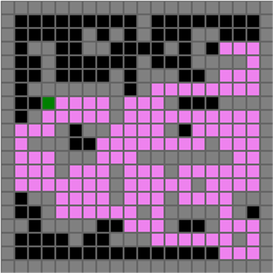
As can be noted, giving a start point ad [_X,_Y] coordinates results in looping through the function (and recursively into it) until all the cells which leads to the solution are crossed. In other words, the algorithm will explore the entire solution domain. Applying the function to our labyrinth, we will obtain a solution like this:
Obviously, that will be an encompassing solution, with the sole purpose of tracking down all possibilities. It is the most dispersive solution. Nonetheless, it could have its usefulness in particular context (please note that, at a conceptual level, our function is a trivial graphical floodfill, given drawing margins), but that's not what we desider to obtain here. We are starting to see wha are the peculiarities of a GA: what it must be able to do? In our case, it must try to solve a labyrinth, without trying to taking out space massively. So, generating individuals capable to solve our problem, we can introduce a kind of limiter.
We saw that limiter above, in the CELLSTATE enumeration, with the value of FakeWall = 5. While we'll generate a new individual, we'll introduce in it some "dirt", to alter the results of the Solve() function with fake walls, precisely, or walls which are not in the base labyrinth structure, having the same behavior of a standard wall
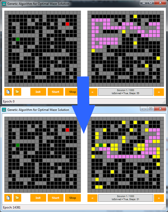
To be spotted more easily, we'll draw them using the yellow color. As said, those are arbitrary limiters, which responds to the same impossability laws as traditional walls, and useful to delimiter, for each reated individual, the solution domain. In fact, we can note that, where a yellow wall is present, the exploration of the maze if blocked from that spot on. Such randomness allows us to generate a manifold population of individuals: it will contain elements that will solve the maze, and elements unable to reach the exit (for example, think about a yellow cell standing right in front of a red one). Next, each solution will arrive to its conclusion in a given number of steps. There will be elements that will arrive to the red cell in a more straight way, while other will follows more convoluted paths, being more dispersive.
An hypothetical solution in VB
Let's now see the code of the GASolver class, which represents the single individual or solution. Please note it has a generic constructor, with a parameter which expects the array of the user-defined maze, to replicate in each solution the bytes representing walls, starting point, end point, which are essential prerequisites to solve the maze, being them fixed. With some probability, one or more cells will take the FakeWall value, to add limiters where - in drawing the maze - the user has left free cells.
Public Class  GASolver

    Dim _startpos(1) As Byte
    Dim _endPos(1) As Byte
    Dim _isSolved As Boolean

    Dim solverBytes(MAZESIZE, MAZESIZE) As Byte

    Public ReadOnly  Property StartPos As Byte()
        Get
            Return _startpos
        End Get
    End Property

    Public ReadOnly  Property EndPos As Byte()
        Get
            Return _endPos
        End Get
    End Property

    Public ReadOnly  Property GetBytes As Byte(,)
        Get
            Return solverBytes
        End Get
    End Property

    Public ReadOnly  Property Steps As Integer
        Get
            Dim _steps As Integer  = 0
            For _Y As Integer  = 0 To  MAZESIZE - 1
                For _X As Integer  = 0 To  MAZESIZE - 1
                    If solverBytes(_X, _Y) = CELLSTATE.Valid Then _steps += 1
                Next
            Next

            Return _steps
        End Get
    End Property

    Public ReadOnly  Property isSolved As Boolean
        Get
            Return Solve(_startpos(0), _startpos(1))
        End Get
    End Property

    Private Function  Solve(_X As  Integer, _Y As Integer) As  Boolean
        If solverBytes(_endPos(0), _endPos(1)) = CELLSTATE.Valid  Then  Return True

        If solverBytes(_X + 1, _Y) = CELLSTATE.Free Or solverBytes(_X + 1, _Y) = CELLSTATE.Start Or solverBytes(_X + 1, _Y) = CELLSTATE.Finish Then
            solverBytes(_X + 1, _Y) = CELLSTATE.Valid
            If Solve(_X + 1, _Y) Then Return  True
        End If

        If solverBytes(_X - 1, _Y) = CELLSTATE.Free Or solverBytes(_X - 1, _Y) = CELLSTATE.Start Or solverBytes(_X - 1, _Y) = CELLSTATE.Finish Then
            solverBytes(_X - 1, _Y) = CELLSTATE.Valid
            If Solve(_X - 1, _Y) Then Return  True
        End If

        If solverBytes(_X, _Y + 1) = CELLSTATE.Free Or solverBytes(_X, _Y + 1) = CELLSTATE.Start Or solverBytes(_X, _Y + 1) = CELLSTATE.Finish Then
            solverBytes(_X, _Y + 1) = CELLSTATE.Valid
            If Solve(_X, _Y + 1) Then Return  True
        End If

        If solverBytes(_X, _Y - 1) = CELLSTATE.Free Or solverBytes(_X, _Y + 1) = CELLSTATE.Start Or solverBytes(_X, _Y + 1) = CELLSTATE.Finish Then
            solverBytes(_X, _Y - 1) = CELLSTATE.Valid
            If Solve(_X, _Y - 1) Then Return  True
        End If

        Return False
    End Function

    Public Sub  New(bytes01(,) As Byte, bytes02(,) As  Byte, startPos As Byte(), endPos As  Byte())
        _startpos = startPos
        _endPos = endPos

        For _Y As Integer  = 0 To  MAZESIZE - 1
            For _X As Integer  = 0 To  MAZESIZE - 1
                If bytes01(_X, _Y) = CELLSTATE.Wall Then solverBytes(_X, _Y) = bytes01(_X, _Y)
                If bytes01(_X, _Y) = CELLSTATE.FakeWall Then solverBytes(_X, _Y) = bytes01(_X, _Y)
            Next
        Next

        For _Y As Integer  = 0 To  MAZESIZE - 1
            For _X As Integer  = 0 To  MAZESIZE - 1
                If bytes02(_X, _Y) = CELLSTATE.Wall Then solverBytes(_X, _Y) = bytes02(_X, _Y)
                If bytes02(_X, _Y) = CELLSTATE.FakeWall Then solverBytes(_X, _Y) = bytes02(_X, _Y)
            Next
        Next

        For _Y As Integer  = 0 To  MAZESIZE - 1
            For _X As Integer  = 0 To  MAZESIZE - 1

                If solverBytes(_X, _Y) <> CELLSTATE.Wall Then
                    Randomize()
                    If Int(Rnd() * 100) Mod 99 = 0 Then
                        If Int(Rnd() * 100) Mod 99 = 0 Then
                            solverBytes(_X, _Y) = CELLSTATE.FakeWall
                        Else
                            solverBytes(_X, _Y) = CELLSTATE.Free
                        End If
                    End If
                End If

            Next
        Next

        solverBytes(startPos(0), startPos(1)) = CELLSTATE.Start
        solverBytes(endPos(0), endPos(1)) = CELLSTATE.Finish
    End Sub

    Public Sub  New(sourceBytes(,) As Byte)
        For _Y As Integer  = 0 To  MAZESIZE - 1
            For _X As Integer  = 0 To  MAZESIZE - 1

                If sourceBytes(_X, _Y) = CELLSTATE.Start Then _startpos(0) = _X : _startpos(1) = _Y
                If sourceBytes(_X, _Y) = CELLSTATE.Finish Then _endPos(0) = _X : _endPos(1) = _Y

                If sourceBytes(_X, _Y) = CELLSTATE.Free Then
                    Randomize()
                    If Int(Rnd() * 100) Mod 50 = 0 Then
                        solverBytes(_X, _Y) = CELLSTATE.FakeWall
                    Else
                        solverBytes(_X, _Y) = CELLSTATE.Free
                    End If
                Else
                    solverBytes(_X, _Y) = sourceBytes(_X, _Y)
                End If

            Next
        Next

    End Sub
End Class
Solve() function is also present, to be able to determine if a solution can reach the exit cell, or if it fails somewhere else. There are other properties and function tht will be analyzed soon.
Solution's fitness
As we saw in the previous article, an essential part of a GA is the one which allows to determine an adaptability score when confronted with a given problem. It goes without saying that the way in which that score will be calculated rests on the problem's tipology. Fitness is essential because, when we have a population made of solution more or less close to our target, it allows to extract some champions with potential characterics we can desire to try ameliorative individual's generation. It is therefore evident that an error in designing a fitness calculator's function will be the foundation stone to build a failure in a GA realization.
In trying to limit problems laying on an eroneous fitness attribution to one or more solutions, deep problem's analyzing is a must. In cases as an image replication is more simple: we know it is - at core - an array of bytes ordered in a given way, and the fitness of a solution passes by checking how many bytes ae shared between our target and the solutions. When confronted with open problems, like the present one, a step forward is needed. Here we aren't interested in evaluating the affinity with a predefined model, but we want to discuss the potential effctiveness of a solution.
Simplifying, in the case of a maze, we are interested in two aspect, already mentioned above:
- The solution must lead to a valid end, it must reach the destination
- The solution must be quick: having satisfied the prerequisite 1), it must be able to obtain it in the most neat way
We can say that, in our case, the fitness calculation passes for two properties: the first is the reach of a goal, while the second is the number of steps taken, where the less is that number, the greater is our solution's quality. To that mean, GASolver class implements two respective properties: isSolver, with returns a boolean value to understand is a particular individual reach the target, and Steps, which count the amount of valid cells in the solution itself.
Initialization and crossing-over
The initialization's concept follows simple rules: is about creating a first generation of solutions, using standard constructors. In the attached source code, the operation happens at the btnInit button's Click:
Private Sub  btnInit_Click(sender As Object, e As  EventArgs) Handles  btnInit.Click
    epochs = 0

    For _Y As Integer  = 0 To  MAZESIZE - 1
        For _X As Integer  = 0 To  MAZESIZE - 1
            If sourceMaze(_X, _Y) = CELLSTATE.Start Then _startPos(0) = _X : _startPos(1) = _Y
            If sourceMaze(_X, _Y) = CELLSTATE.Finish Then _endPos(0) = _X : _endPos(1) = _Y
        Next
    Next

    gaList = New  List(Of GASolver)
    For ii As Integer  = 0 To  999
        gaList.Add(New GASolver(sourceMaze))
    Next

    gaCursor = 0
    MazePaintItem(mazeDest)

    btnStart.Enabled = True
    btnStop.Enabled = False
End Sub
We reset a counter which will be used to count generations, then we save the cells which the user has defined as the start and end point. In a List(OF GASolver), which we will query via LINQ, we'll add the desired number of newly created GASolver (in our case, 1000 units), to proced to their graphical representation. Each initial solution, as we saw, will be initialized adding dummy limiters into the spaces the user has kept clear, to create variety into population.
By pressing btnStart button, the seach for solutions will start. Note that we will extract at each loop those elements which solve the maze (ga.isSolved = True), ordered by the number of steps used to complete the task (Order By ga.Steps Ascending). That way, we will be sure to extract the two best solutions at the moment. Those elements will be recombined, producing two new elements, following the rules we'll see in a moment. Lastly, ordering our list for a descending amount of steps, we can discard the two worst elements. Please note that we won't apply any discriminant on the solution's quality, and it is possible to discard elements which comes to a valid solution, but having the flaw to be - among all solutions - the most dispersive ones.
Cross-over generating the two new elements is explained through the four-argument constructor of GASolver class, as follows:
Public Sub  New(bytes01(,) As Byte, bytes02(,) As  Byte, startPos As Byte(), endPos As  Byte())
    _startpos = startPos
    _endPos = endPos

    For _Y As Integer  = 0 To  MAZESIZE - 1
        For _X As Integer  = 0 To  MAZESIZE - 1
            If bytes01(_X, _Y) = CELLSTATE.Wall Then solverBytes(_X, _Y) = bytes01(_X, _Y)
            If bytes01(_X, _Y) = CELLSTATE.FakeWall Then solverBytes(_X, _Y) = bytes01(_X, _Y)
        Next
    Next

    For _Y As Integer  = 0 To  MAZESIZE - 1
        For _X As Integer  = 0 To  MAZESIZE - 1
            If bytes02(_X, _Y) = CELLSTATE.Wall Then solverBytes(_X, _Y) = bytes02(_X, _Y)
            If bytes02(_X, _Y) = CELLSTATE.FakeWall Then solverBytes(_X, _Y) = bytes02(_X, _Y)
        Next
    Next

    For _Y As Integer  = 0 To  MAZESIZE - 1
        For _X As Integer  = 0 To  MAZESIZE - 1

            If solverBytes(_X, _Y) <> CELLSTATE.Wall Then
                Randomize()
                If Int(Rnd() * 100) Mod 99 = 0 Then
                    If Int(Rnd() * 100) Mod 99 = 0 Then
                        solverBytes(_X, _Y) = CELLSTATE.FakeWall
                    Else
                        solverBytes(_X, _Y) = CELLSTATE.Free
                    End If
                End If
            End If

        Next
    Next

    solverBytes(startPos(0), startPos(1)) = CELLSTATE.Start
    solverBytes(endPos(0), endPos(1)) = CELLSTATE.Finish
End Sub
Essentially, it requires two arrays, referred to the bytes of the elements to be recombined, and two pairs of coordinates, namely the start and exit point of the maze.
Looping through the two matrices, a resultant matrix is generated, putting in it the combination of Wall and FakeWall types. Wall cell will be the same between the two, but FakeWall will possibily differ. If the two solutions come to a valid end, it means the FakeWall from both matrices can be applied without affect the solution, making it better by remove potential free cell to be considered valid steps. When the process ends, an additional mutation loop calculates the eventual transformation of non-Wall cells in Wall or FakeWall cells. The newly created solution will then have the same Walls as parents, the same start/end point, but the virtual walls from both, plus some mutation (if they will occur).
The logic is simple: the thing which determines a more economic solution, is the freedom of movement. The more the free cells are, the greater the solution's domain will be and - consequently - the steps towards the exit point. In the described way, we apply a progressive limiter towards a basic path, which will be constituted by the sum of the limiters which - in past generations - had represented and help to that mean.
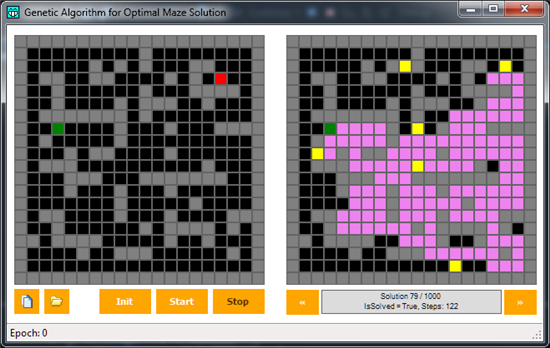
Making the algorithm run, alternating generations, in a few hundreds of epochs we'll have the optimal solution, or the solution which leads from start point to end without "indecisions". At the same time, the progressive discarding of poor solutions, in favor of those with higher performances, will lead to an entire population of acceptable solutions.
In the above example, it's possible to see that after about 14000 generations of solutions, the result is really close to the optimal one: there is room to improve, and proceeding though epochs it's possible to reach better results, though with the slowness due to recombination of nearly-ideal solutions (which can count almost exclusively on mutation to improve further). Lastly, please note that - with a given number of potential solutions - the path chosen by the algorithm will be affected by the elaborations themselves: for example, if a mutation inhibits a certain path, the algorithm will focus on remaining solutions. So, we won't obtain the ultimately better overall solution, but the better according to the current context, and the agents at our disposal, miming at a conceptual level what happens in biology too.
Source Code
Demo
A sample video about a session from the program is available here:
References
- http://en.wikipedia.org/wiki/DNA
- http://en.wikipedia.org/wiki/Natural_selection
- http://en.wikipedia.org/wiki/Genetic_algorithm
- Genetic algorithm for icon generation in Visual Basic
Other Languages
This article is also available in Italian. Please check:
