Excel: How to filter a report using a list of comma-separated strings
In Excel, we have a table which has a column in it containing a string of Comma Separated Values (CSV) e.g. VALUE1, VALUE2, VALUE3.
Each row can have one or more values under this column.
Now for all the values under this column, we need to create a filter that can be used in Power Pivot or Power View.
There is a simple procedure for doing this from within Excel, using a simple transformation via Power Query (earlier called Data Explorer), using the following steps:
1. Download and install Power Query
Power Query is a free add-in tool, used for simplifying data discovery and access. It is available for download here: http://office.microsoft.com/en-us/excel/download-microsoft-power-query-for-excel-FX104018616.aspx
Once installed, the Power Query menu would be available in the Menu Ribbon.
2. Open the Excel table
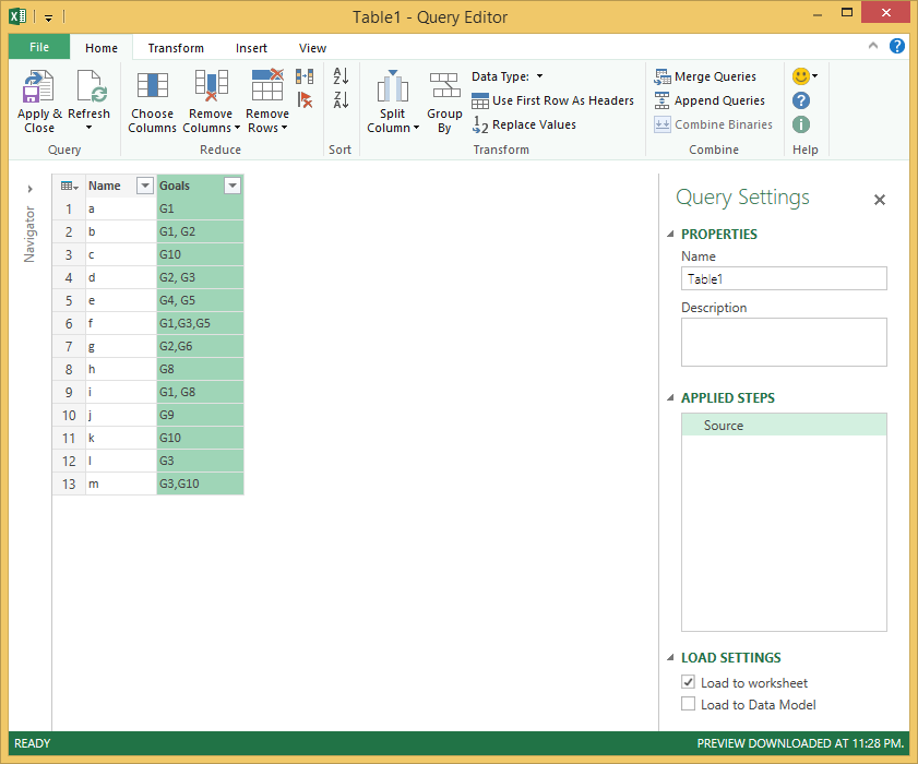
Open the Excel table which contains the data to be transformed, and click on any cell within the table. In our case, we have a table with some names, and goals associated with each name. Here we would need to transform the table such that each single row will have a single value for goal.
3. Power Query
From the menu ribbon, select ‘POWER QUERY’ > ‘From Table’ (under the Excel Data group).
This would open a new Query Editor window.
4. Edit query
In the query editor window will have a main area, having our table, and a Query Settings pane, which lists the key properties of this query, and the steps applied during this query. It also provides options to load the transformed data directly into a new worksheet, or into the Excel Data Model.
5. Split colum by delimiter
Right Click on the column header ‘Goals’, and select ‘Split Column’ > ‘By Delimiter’.
6. Select comma
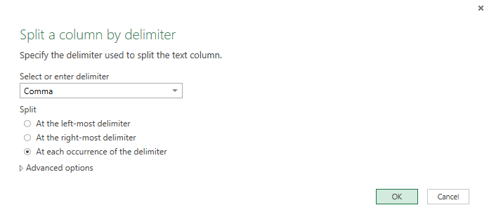
From the window ‘split column by delimiter’ select ‘Comma’ from the drop-down list, and from the split radio button, select the last radio button ‘At each occurrence of the delimiter’. Then click 'Ok'.
This would split the Goals column into multiple columns. The number of new column would be equal to the maximum number of comma separated values in a single row. In our case, since row 6 has three values (G1, G3 and G5) we get three columns.
7. Unipivot
Select all the newly created columns by pressing ‘Shift + click on column headers’. When all three columns are selected, right click on any one column header, and select ‘Unpivot’.
8. Remove colums
The table would get many additional rows, with all selected columns rolling up into two columns. The values in the attribute is not required, so we can delete this column by selecting “Home” > “Remove Columns” > “Remove Columns” option.
9. Trim
The column ‘Values’ has many cells will have additional blank spaces before and after the actual values. We can trim them by right clicking on the column header, and selecting “Transform” > “Trim” option.
In the query settings pane, provide the appropriate values for name and description. All the steps performed during this transformation can be seen under ‘APPLIED STEPS’. Also, the options for adding the table to worksheet or the Excel Data model can be selected as desired.
10. Apply and close
Once all changes are made, the table can be saved using the “Home” > “Apply and Close” option.
11. Filtering
The desired data would be now available in form of a new table. The ‘Value’ column of this table can be used in any power Pivot or Power View query for filtering all the relevant names for corresponding values of goals.
Download
The sample Excel sheet with this transformation is available on the TechNet Gallery here:
Download the sample Excel sheet from here:
Filtering a report in Excel using a list of comma-separated strings


