Note
Access to this page requires authorization. You can try signing in or changing directories.
Access to this page requires authorization. You can try changing directories.
Note: Here's a more current topic about working with Dates in PowerPivot.
For more information, read:
The PowerPivot for Excel 2010 overview.
or
The PowerPivot for Excel 2013 overview.
When you create a PivotTable that is based on Excel data, you can group the data in the PivotTable. For example, the source data for a PivotTable might contain a column that stores the date of the sale, but you can also see the data grouped by quarters or months, rather than days.
Note: You can use grouping for other types of data, but I will focus on dates here.
Original article (before wiki edits) was written by Michael Blythe, Microsoft SQL Server Analysis Services Content Publishing Manager.
The following screenshots show the Grouping dialog box and the effect of grouping by months.

You can see that the table in the Field List has only a Sales Date column, but the PivotTable is now sorted by month – Excel interprets the dates and provides this ability to group by different time periods. This Excel feature is not supported for PivotTables that are based on PowerPivot data, but you can achieve the same effect by adding columns to your source table. If your source table already has columns that represent the grouping that you need, then skip to the end of this article to see a screenshot of a PivotTable that shows PowerPivot data grouped by months.
Here’s the data that was used for the Excel PivotTables in the screenshots above:
| Sales ID | Sales Date | Store Name | Product Name | Sales Amount |
| 182 | 11/11/2007 | Contoso Lancashire Store | WWI Laptop15 M0150 Black | $5,032.80 |
| 235 | 9/26/2007 | Contoso West Yorkshire Store | Contoso Home Theater System 5.1 Channel M1530 Black | $3,471.30 |
| 394 | 5/31/2008 | Contoso Lancashire Store | Contoso USB Optical Mouse E200 White | $155.00 |
| 431 | 11/13/2007 | Contoso Baildon Store | Proseware Fax Machine E100 White | $252.80 |
| 488 | 8/24/2009 | Contoso Cambridge Store | Proseware Ink Jet Instant PDF Sheet-Fed Scanner M300 Grey | $1,888.00 |
| 599 | 9/10/2008 | Contoso Cambridge Store | Proseware Color Ink jet Fax, Copier, Phone M250 White | $1,844.40 |
| 654 | 7/6/2009 | Contoso London Store | Contoso Home Theater System 2.1 Channel M1230 White | $3,600.00 |
| 683 | 8/14/2007 | Contoso Leeds Store | Adventure Works CRT19 E10 White | $248.40 |
| 786 | 1/12/2009 | Contoso Edinburgh Store | Fabrikam Laptop17 M7000 Black | $5,896.80 |
| 795 | 6/10/2007 | Contoso Cheshire Store | Proseware Scan Jet Digital Flat Bed Scanner M300 White | $1,210.00 |
| 854 | 11/15/2007 | Contoso Cheshire Store | Proseware High-Speed Laser M2000 White | $4,765.20 |
| 918 | 8/1/2009 | Contoso Leeds Store | Adventure Works Laptop12 M1201 Red | $6,854.81 |
| 970 | 10/1/2009 | Contoso Cheshire Store | Contoso Home Theater System 4.1 Channel M1400 Black | $3,026.60 |
| 1084 | 11/20/2009 | Contoso Knotty Ash Store | Proseware CRT19 E201 White | $1,076.40 |
| 1187 | 2/28/2007 | Contoso London Store | Contoso Ultraportable Neoprene Sleeve E30 Yellow | $93.60 |
| 1379 | 9/13/2008 | Contoso Edinburgh Store | Adventure Works Laptop15 M1501 Red | $6,081.30 |
| 1457 | 2/26/2007 | Contoso Manchester Store | Proseware Ink Jet Fax Machine E100 Black | $462.54 |
| 1494 | 1/31/2008 | Contoso Baildon Store | WWI Screen 100in M1609 Black | $1,444.00 |
| 1761 | 2/1/2007 | Contoso Liverpool Store | Adventure Works Desktop PC1.80 ED182 White | $17,926.41 |
| 1817 | 12/15/2007 | Contoso York Store | Litware Home Theater System 2.1 Channel E212 Black | $959.68 |
This is a small table, so you could just manually add columns for whatever time periods you want (such as a Month column) and fill them out with data for each row. But a lot of times this is not practical, so I will show you how to group by using calculated columns in the PowerPivot window. These calculated columns use Data Analysis Expressions (DAX), which is similar to the Excel function language. For more information, see Getting Started with DAX and Create a Calculated Column in the PowerPivot Help on TechNet Library.
To start: copy the table above, paste it into the PowerPivot window, and name it Sales. For information about pasting data into PowerPivot, see Copy and Paste Data in the PowerPivot Help.
Now that you have the data in PowerPivot, add a calculated column with the following DAX formula, then right-click the column, and rename it MonthNumber:
=MONTH(Sales[Sales Date])
Like in Excel, this function returns the month number (such as 2) not the name (such as February). If you only want to group by months and the month number is sufficient, you can stop here. If you want to expand on this a little more, you can add a lookup table that allows you to pull different values into the Sales table:
| MonthNumber | MonthShortName | MonthFullName | Quarter | Semester |
| 1 | Jan | January | Q1 | H1 |
| 2 | Feb | February | Q1 | H1 |
| 3 | Mar | March | Q1 | H1 |
| 4 | Apr | April | Q2 | H1 |
| 5 | May | May | Q2 | H1 |
| 6 | Jun | June | Q2 | H1 |
| 7 | Jul | July | Q3 | H2 |
| 8 | Aug | August | Q3 | H2 |
| 9 | Sep | September | Q3 | H2 |
| 10 | Oct | October | Q4 | H2 |
| 11 | Nov | November | Q4 | H2 |
| 12 | Dec | December | Q4 | H2 |
Copy the table above, paste it into the PowerPivot window, and name it TimePeriods. Now add a relationship between the two tables, using the Sales[MonthNumber] and TimePeriods[MonthNumber] columns. For information about creating relationships, see Create a Relationships Between Two Tables in the PowerPivot Help.
The time period's table illustrates a way that you can handle grouping. You can also build a more general purpose date/time table, such as the one described here on the PowerPivot-Info Web site.
Now that the tables are related to each other, you can easily use data from the time period's table in the Sales table. Add a calculated column with the following formula and rename the column Month:
=RELATED(TimePeriods[MonthShortName])
You can see how the RELATED function pulls in the short month name by following the relationship that you created between the two tables. Months will sort alphabetically in the PivotTable, so if you use this formula as-is, Aug will end up first. To avoid this, update the formula as follows, which adds the date number with a leading zero so that it sorts correctly:
= "(" & IF(Sales[MonthNumber] < 10,"0","") & Sales[MonthNumber] & ")" & " " & RELATED(TimePeriods[MonthShortName])
Sales for February will now appear in a PivotTable under the heading (02) Feb.
You can now add two more columns –Quarters and Years – with the following formulas:
=RELATED(TimePeriods[MonthQuarterName])
=YEAR(Sales[Sales Date])
Like the MONTH formula I showed earlier, the YEAR formula can get what it needs from the Sales Date column and doesn’t require the TimePeriods table.
The formulas shown above are one way to tackle this problem, but the specific approach is less important than the general principle of finding an easy way to add the time period columns that you need for grouping. After you have added those columns, you can create a PivotTable based on the data and group it based on which columns you select from the PowerPivot Field List.
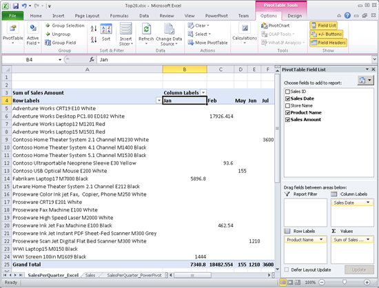
Create a PivotTable from the PowerPivot window. For information about creating a PivotTable, see this video on the Business Intelligence TechNet page. In the Field List, drag Sales Date to the Column Labels pane, Product Name to Row Labels, and Sales Amount to Values. Now clear the Sales Date column and drag the Month column to Column Labels instead.
As you can see in the following screenshot, data is now grouped by months.

Original article (before wiki edits) was written by Michael Blythe, Microsoft SQL Server Analysis Services Content Publishing Manager.
See Also