Partitioning & Archiving tables in SQL Server (Part 1: The basics)
Database partitioning is a feature available in SQL Server(version 2005 and Up) which lets you split a table among multiple files which can be beneficial for large tables, especially for those which hold historical data. Using partitioning You can also simplify data management ( like storage size and placement, backups strategy etc.) as well as index management, making queries run faster when working with smaller ranges of data. Data partitioning is really easy to implement if you clearly understand how it works and if you plan your strategy carefully. You can also benefit from this feature to archive old data in a very easy way.
You can find much information about data partitioning on the Internet including the examples from MSDN and BOL, however there are important considerations you must care about and experiment with different data scenarios before implementing data partitioning in a production environment. This article focuses on these topics as well as partition management including split and merge partitions and the switch partition option.
Filegroups and Data Files
As you know, a database contains a data file (.MDF) and a transaction log file (.LDF), however you can add additional files to the database,these files are called secondary files (.NDF) and can be also use to store data rows. The files are assigned to filegroups in the same way the files are assigned to folders in the a file system, however, when assign several files to the same filegroup, data is distributed evenly between all of them, in a round-robin way.To begin the example, let´s create a sample database called PartitionDB with 3 filegroups and 3 additional files (.NDF).
In SQL Server Management Studio, right click on Databases –> New Database. You can add the filegroups in the Filegroups page or you can add the files (.NDF) in the Files page and add the filegroup at the same time in the Files page. Just go to Files Page, click the Add Button, in the Logical Name column, type a name for the File, click on Filegroup column, select <new Filegroup> and type a name for the filegroup:
Define partitions
Now, we need decide how to partition our data. Is different the scenario where you want to partition a table which already contains data from a scenario where you are creating a new table. In the first case, you must be aware of the primary key in terms of how is build, which column (s) participate and the data types, you must also care about the unique index which the Primary key builds automatically . In the case you are building a new table from scratch, you can decide how to create the table, the primary key and the partitioning strategy, in the first case you will be limited to what the table design allows.
In this examples we are going to create 2 new tables, the tables will simulate order information. The first example will implement partitioning by using OrderID as the partition column while the second example will use OrderDate. The partition column is called Partition Key and represents the criteria used to partition the information.
Partition Function
The partition function creates the ranges of data (partitions) according to values defined inside its body. This values are the boundaries which in turn produce the ranges. The function takes a data type as a parameter according to the column you selected as the partition key. When you define the boundaries for the partitions, you can use RIGHT or LEFT to define the limits of each partition.
LEFT means each value represents the upper limit for each range, in other words, each range goes from each boundary value to the LEFT.
RIGHT means each value represent the lower limit for each range but the first range will start to the right of the first value, so there will be an additional range (the first range) and the first boundary value in the function defines where the second range begins.
To better understand, suppose you have 10 000 records and want to create 3 ranges, the first range goes from 1-1000, the second from 1001 to 5000 and the third from 5001 to 10000. Since the partitions are based on numbers, you should pass a numeric datatype as an argument to the function.
Let´s create a function named pfRecordsRange in order to do this:
Note that the function uses LEFT for defining ranges, as I said before when using left each value represents the upper limit. 1000 is the upper limit for the first range, 5000 for the second and 10000 for the third.
If the first record starts in 1, this would be the lower limit for the first range (1-1000) , 10001 would be the lower limit for the second range (1001 – 5000) and 5001 for the 3rd (5001 – 10 000)
But look, what if more records are inserted outside the limits? for example where would the record 10001 be placed?
well, in fact another range is automatically generated for all the records that are greater than the last value defined in the function (>10000) and this will be the last range, so the record 10001 will be placed here.
Another question: If the value –1 would be inserted, where would it be placed?. The answer is: In the first range.
In fact the first and the last ranges have no limits, both have just one boundary, so consider to add a check constraint in your table to restrict the values that can be inserted in these ranges.
Another important consideration: You will need an additional filegroup to hold the data for the additional range. You will always need to consider 1 additional filegroup apart from those required by the function values. If your function includes n values, you will need n+1 filegroups.
This requirement is just to be sure the function will be able to place each partition in an available filegroup but it does not really mean there will be data for the last filegroup, so you could use the PRIMARY file group as the target for the last partition.
Returning to our example, If I use RIGHT instead of LEFT the first boundary value (1000) in the function would be the lower limit for the second range and the first range would include all records which are less than 1000, the last range would include the number 10000, that is mean >=10000.
The following image shows the difference when using LEFT and RIGHT in terms of the ranges they produce:
If LEFT is used, the first value in the function will be part of the first partition. If RIGHT is used, it will be part of the second partition, also look how the ranges are defined in each case. So, the only difference is the partition each value belongs to. The symblos <,<=,>,>=, define this boundaries.
Right or Left?
This is a common question, and the answer is: it all depends how you want to define your partitions, In my case, when I work with numeric ranges I prefer to use LEFT because usually I´ll want to include the upper limit in each range (1 to 10,, 11 to 20, etc.) however when I work with dates I prefer to use RIGHT because I prefer to define ranges by the start date not by the end date, for example If I want 3 partitions for each year (one for 2009, another for 2010 and the last for 2011) is easier to consider the start value for each range: 2009/01/01, 2010/01/01, etc. instead of the end range. Look at the script for this partition function:
Partition Schema
Once you have created the partition function, the next step is creating the partition schema. The partition schema uses the partition function to redirect the partitions defined by the function to the appropriate filegroups. Remember, if you have 3 values defined in the function it will produce 4 ranges (partitions).
In this case, assume we want a partition schema for the function pfOrderDateRange.
The schema would looks like this:
Note that I used PRIMARY for the last filegroup since no data will be stored here.
Partitioned Table
The last step is creating the table using the partition schema to store data in a partitioned fashion. When you create a table, you can define where to store the table (CREATE TABLE <name> (…) ON ). If you omit the ON part of the statement, the table will be created on the default filegroup which is usually the PRIMARY filegroup. In this case, we will tell the table to store the data in several partitions which is the job of the partition schema, so simply put the partition schema name after the ON clause and add the column name as the argument.
Before showing the script let´s talk about the primary key column.
When you add a primary key constraint to a table an index is also built on this column. The index may be clustered or non clustered (you can choose) but it must be unique. This unique index is used is to reinforce rows uniqueness. We will not discuss index structures here but remember this: if the Primary Key contains a clustered index, the table will be sorted using the index column (or columns). I f the Primary Key contains a non clustered index, an additional sorted structure will be created and the table data will remain as is.
Index and Data Alignment
The best practice when creating a partitioned table is to partition the index the same way you partition the data, this is called aligned index. But to be able to align index to data rows you must include the partition key (the column by which you are partitioning) in the index definition. If you do this, each index portion will be stored in the same data file (.ndf) where the corresponding data portion is stored, this way, if you query a table using a range expression (WHERE order date BETWEEN…), SQL Server will only use the corresponding index data for the query. The execution plan will be more efficient. Also, you can backup filegroups and create a more efficient recovery strategy because index are contained in the same filegroup. When indexes are aligned, You can move a partition to another table without moving rows just the metadata in just seconds!. It is highly recommended align indexes in order to benefit from this features.
Since this is the best scenario possible, lets create a primary Key for our table (orders) using OrderID as well as OrderDate which is the partition key. Look at the script:
That´s all, now when you insert data into your table, each row is evaluated using the partition function to identify the corresponding partition, Partition schema will store the data to the corresponding filegroup using the partition function and the index will be stored in the same filegroups as the corresponding data.
Populate and Verify Data
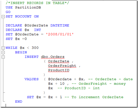
Now let´s insert some rows in our table using this simple script:
I´ll run the script tree times, each using the values ‘2008/01/01’, ‘2009/01/01’ and ‘2010/01/01’ for the @OrderDate variable in order to insert 900 rows.
Finally, use the following script which uses the transact $PARTITION to verify how many rows are inserted in each partition as well as the data boundaries:
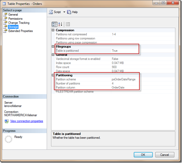
You can also view the table properties to verify data partitioning:
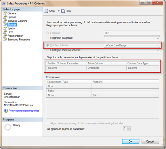
And look at the index properties:
If you wish, you can create the following view (taken from SQL Server 2008 Internals by Kalen Delaney, Paul S. Randal, Kimberly L. Tripp, and Conor Cunningham):
and then query the view to obtain the following results:
This view is similar to the other query but is very useful because you can also see the name of the filegroup and the name of the table where each partitions is stored, you will appreciate this information when merging and splitting data, without this info, is difficult to see where the data was moved.
This is the simplest procedure for data partitioning, in the next post I´ll talk about split and merge data, and what to do when you can’t align indexes as well as other scenarios.
Comments
Anonymous
February 06, 2012
This is the most useful article I have come across regarding partitioning. Great job and thanks for clearly explaining the basicsAnonymous
February 14, 2012
Thanks for your comments Bob, that´s why I like to share :)Anonymous
February 23, 2012
I've been reading about partitioning all day and I finally understand the difference between the 'right' and 'left' boundaries. Thanks for the detail and multiple examples!Anonymous
February 28, 2012
Thank you, a very good introductionAnonymous
July 02, 2012
Awesome !Anonymous
October 15, 2012
This is a very helpful articleAnonymous
October 18, 2012
Excellent explanation of paritioning. Thank you!Anonymous
November 06, 2012
Great Article, however, code should have been copy past friendly, instead of just screen shots. Again, thanks for the great article.Anonymous
August 22, 2013
very helpful example easily understandableAnonymous
October 16, 2013
Some cases we can't go with partition. You can use dynamic approach of archiving and purging data in SQL Server. Please follow below link for that. www.sqlscientist.com/.../auto-maintain-archival-process.htmlAnonymous
November 19, 2013
Thanks a lot Felix :) I appreciate it.Anonymous
December 04, 2013
Just another now-well-informed user. Your explanation is the gold standard on LEFT vs RIGHT with your great query on partition usage. Copy/Paste friendly version: SELECT OBJECT_NAME(i.object_id) AS OBJECT_NAME, p.partition_number, fg.NAME AS FILEGROUP_NAME, ROWS, au.total_pages, CASE boundary_value_on_right WHEN 1 THEN 'Less than' ELSE 'Less or equal than' END AS 'Comparison', VALUE FROM sys.partitions p JOIN sys.indexes i ON p.object_id = i.object_id AND p.index_id = i.index_id JOIN sys.partition_schemes ps ON ps.data_space_id = i.data_space_id JOIN sys.partition_functions f ON f.function_id = ps.function_id LEFT JOIN sys.partition_range_values rv ON f.function_id = rv.function_id AND p.partition_number = rv.boundary_id JOIN sys.destination_data_spaces dds ON dds.partition_scheme_id = ps.data_space_id AND dds.destination_id = p.partition_number JOIN sys.filegroups fg ON dds.data_space_id = fg.data_space_id JOIN ( SELECT container_id, SUM(total_pages) AS total_pages FROM sys.allocation_units GROUP BY container_id ) AS au ON au.container_id = p.partition_id WHERE i.index_id < 2Anonymous
May 12, 2014
Great Post!!!Anonymous
September 03, 2014
Owsome... Great article... Very useful...Anonymous
December 09, 2014
The comment has been removedAnonymous
January 08, 2015
great article, this is also a great guide about using a SQL Server distributed partitioned view to allow transparent querying of multiple Azure SQL databasesp sqlturbo.com/tutorial-how-to-query-multiple-azure-sql-databases-transparently-from-one-on-premise-sql-serverAnonymous
February 02, 2015
Nice article. Keep up the good work.Anonymous
June 24, 2015
very good introduction,thank u very much:) http://playgamenow.me/Anonymous
September 08, 2015
Awesome articles! That's more helpful than any books from MS. Thanks so much!Anonymous
November 02, 2015
There is no mention of any archiving in the article. It explains partioning nicely. But how does one detach older partitions and possibly back them up on addition storage and then if need be reattach them?Anonymous
December 16, 2015
Very helpful document! I've found the [dbo].[Partition_Info] view text on github for those who don't want to type it out: github.com/.../partition_info_view.sqlAnonymous
June 06, 2016
One of the best examples explained very briefly .Anonymous
February 23, 2017
Excellent article. Thanks for sharing. I just suggest to add the compatible version which is the Enterprise Edition at the top of the article.


