Build an R model and save to SQL Server (walkthrough)
Applies to:
SQL Server 2016 (13.x) and later versions
In this step, learn how to build a machine learning model and save the model in SQL Server. By saving a model, you can call it directly from Transact-SQL code, using the system stored procedure, sp_execute_external_script or the PREDICT (T-SQL) function.
Prerequisites
This step assumes an ongoing R session based on previous steps in this walkthrough. It uses the connection strings and data source objects created in those steps. The following tools and packages are used to run the script.
- Rgui.exe to run R commands
- Management Studio to run T-SQL
- ROCR package
- RODBC package
Create a stored procedure to save models
This step uses a stored procedure to save a trained model to SQL Server. Creating a stored procedure to perform this operation makes the task easier.
Run the following T-SQL code in a query windows in Management Studio to create the stored procedure.
USE [NYCTaxi_Sample]
GO

SET ANSI_NULLS ON
GO
SET QUOTED_IDENTIFIER ON
GO

IF EXISTS (SELECT * FROM sys.objects WHERE type = 'P' AND name = 'PersistModel')
  DROP PROCEDURE PersistModel
GO

CREATE PROCEDURE [dbo].[PersistModel] @m nvarchar(max)
AS
BEGIN
	-- SET NOCOUNT ON added to prevent extra result sets from
	-- interfering with SELECT statements.
	SET NOCOUNT ON;
	insert into nyc_taxi_models (model) values (convert(varbinary(max),@m,2))
END
GO
Note
If you get an error, make sure that your login has permission to create objects. You can grant explicit permissions to create objects by running a T-SQL statement like this: exec sp_addrolemember 'db_owner', '<user_name>'.
Create a classification model using rxLogit
The model is a binary classifier that predicts whether the taxi driver is likely to get a tip on a particular ride or not. You'll use the data source you created in the previous lesson to train the tip classifier, using logistic regression.
Call the rxLogit function, included in the RevoScaleR package, to create a logistic regression model.
system.time(logitObj <- rxLogit(tipped ~ passenger_count + trip_distance + trip_time_in_secs + direct_distance, data = featureDataSource));The call that builds the model is enclosed in the system.time function. This lets you get the time required to build the model.
After you build the model, you can inspect it using the
summaryfunction, and view the coefficients.summary(logitObj);Results
 *Logistic Regression Results for: tipped ~ passenger_count + trip_distance + trip_time_in_secs +*
 direct_distance*
 *Data: featureDataSource (RxSqlServerData Data Source)*
 *Dependent variable(s): tipped*
 *Total independent variables: 5*
 *Number of valid observations: 17068*
 *Number of missing observations: 0*
 *-2\*LogLikelihood: 23540.0602 (Residual deviance on 17063 degrees of freedom)*
 *Coefficients:*
 *Estimate Std. Error z value Pr(>|z|)*
 *(Intercept)       -2.509e-03  3.223e-02  -0.078  0.93793*
 *passenger_count   -5.753e-02  1.088e-02  -5.289 1.23e-07 \*\*\**
 *trip_distance     -3.896e-02  1.466e-02  -2.658  0.00786 \*\**
 *trip_time_in_secs  2.115e-04  4.336e-05   4.878 1.07e-06 \*\*\**
 *direct_distance    6.156e-02  2.076e-02   2.966  0.00302 \*\**
 *---*
 *Signif. codes:  0 '\*\*\*' 0.001 '\*\*' 0.01 '\*' 0.05 '.' 0.1 ' ' 1*
 *Condition number of final variance-covariance matrix: 48.3933*
 *Number of iterations: 4*
Use the logistic regression model for scoring
Now that the model is built, you can use to predict whether the driver is likely to get a tip on a particular drive or not.
First, use the RxSqlServerData function to define a data source object for storing the scoring result.
scoredOutput <- RxSqlServerData(
  connectionString = connStr,
  table = "taxiScoreOutput"  )
To make this example simpler, the input to the logistic regression model is the same feature data source (
sql_feature_ds) that you used to train the model. More typically, you might have some new data to score with, or you might have set aside some data for testing vs. training.The prediction results will be saved in the table, taxiscoreOutput. Notice that the schema for this table is not defined when you create it using rxSqlServerData. The schema is obtained from the rxPredict output.
To create the table that stores the predicted values, the SQL login running the rxSqlServer data function must have DDL privileges in the database. If the login cannot create tables, the statement fails.
Call the rxPredict function to generate results.
rxPredict(modelObject = logitObj,
    data = featureDataSource,
    outData = scoredOutput,
    predVarNames = "Score",
    type = "response",
    writeModelVars = TRUE, overwrite = TRUE)
If the statement succeeds, it should take some time to run. When complete, you can open SQL Server Management Studio and verify that the table was created and that it contains the Score column and other expected output.
Plot model accuracy
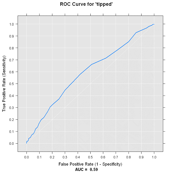
To get an idea of the accuracy of the model, you can use the rxRoc function to plot the Receiver Operating Curve. Because rxRoc is one of the new functions provided by the RevoScaleR package that supports remote compute contexts, you have two options:
You can use the rxRoc function to execute the plot in the remote compute context and then return the plot to your local client.
You can also import the data to your R client computer, and use other R plotting functions to create the performance graph.
In this section, you'll experiment with both techniques.
Execute a plot in the remote (SQL Server) compute context
Call the function rxRoc and provide the data defined earlier as input.
scoredOutput = rxImport(scoredOutput);
rxRoc(actualVarName= "tipped", predVarNames = "Score", scoredOutput);
This call returns the values used in computing the ROC chart. The label column is tipped, which has the actual results you are trying to predict, while the Score column has the prediction.
To actually plot the chart, you can save the ROC object and then draw it with the plot function. The graph is created on the remote compute context, and returned to your R environment.
scoredOutput = rxImport(scoredOutput);
rocObjectOut <- rxRoc(actualVarName= "tipped", predVarNames = "Score", scoredOutput);
plot(rocObjectOut);
View the graph by opening the R graphics device, or by clicking the Plot window in RStudio.

Create the plots in the local compute context using data from SQL Server
You can verify the compute context is local by running rxGetComputeContext() at the command prompt. The return value should be "RxLocalSeq Compute Context".
For the local compute context, the process is much the same. You use the rxImport function to bring the specified data into your local R environment.
scoredOutput = rxImport(scoredOutput)Using the data in local memory, you load the ROCR package, and use the prediction function from that package to create some new predictions.
library('ROCR');
pred <- prediction(scoredOutput$Score, scoredOutput$tipped);
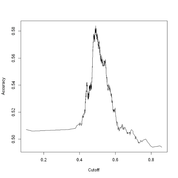
Generate a local plot, based on the values stored in the output variable
pred.acc.perf = performance(pred, measure = 'acc'); plot(acc.perf); ind = which.max( slot(acc.perf, 'y.values')[[1]] ); acc = slot(acc.perf, 'y.values')[[1]][ind]; cutoff = slot(acc.perf, 'x.values')[[1]][ind];
Note
Your charts might look different from these, depending on how many data points you used.
Deploy the model
After you have built a model and ascertained that it is performing well, you probably want to deploy it to a site where users or people in your organization can make use of the model, or perhaps retrain and recalibrate the model on a regular basis. This process is sometimes called operationalizing a model. In SQL Server, operationalization is achieved by embedding R code in a stored procedure. Because code resides in the procedure, it can be called from any application that can connect to SQL Server.
Before you can call the model from an external application, you must save the model to the database used for production. Trained models are stored in binary form, in a single column of type varbinary(max).
A typical deployment workflow consists of the following steps:
- Serialize the model into a hexadecimal string
- Transmit the serialized object to the database
- Save the model in a varbinary(max) column
In this section, learn how to use a stored procedure to persist the model and make it available for predictions. The stored procedure used in this section is PersistModel. The definition of PersistModel is in Prerequisites.
Switch back to your local R environment if you are not already using it, serialize the model, and save it in a variable.
rxSetComputeContext("local");
modelbin <- serialize(logitObj, NULL);
modelbinstr=paste(modelbin, collapse="");
Open an ODBC connection using RODBC. You can omit the call to RODBC if you already have the package loaded.
library(RODBC);
conn <- odbcDriverConnect(connStr);
Call the PersistModel stored procedure on SQL Server to transmit the serialized object to the database and store the binary representation of the model in a column.
q <- paste("EXEC PersistModel @m='", modelbinstr,"'", sep="");
sqlQuery (conn, q);
Use Management Studio to verify the model exists. In Object Explorer, right-click on the nyc_taxi_models table and click Select Top 1000 Rows. In Results, you should see a binary representation in the models column.
Saving a model to a table requires only an INSERT statement. However, it's often easier when wrapped in a stored procedure, such as PersistModel.
Next steps
In the next and final lesson, learn how to perform scoring against the saved model using Transact-SQL.