Demand forecasting algorithms

Demand planning in Microsoft Dynamics 365 Supply Chain Management includes four popular demand forecasting algorithms: auto-ARIMA, ETS, Prophet, and XGBoost.

• Auto-ARIMA is suited for stationary data. Stationary data is data that has constant mean, constant standard deviation, and no seasonality.
• Error, trend, and seasonality (ETS) excels if your business case is simple and the data has various patterns, such linear or exponential trends, or if you want the forecast to give more weight to the most recent data.
• Prophet works best with complex, real-world data.
• eXtreme Gradient Boosting (XGBoost) can generate a forecast based on two inputs.

In addition, Demand planning provides a best fit model algorithm, which automatically selects the best of the available algorithms for each product and dimension combination. Demand planning also lets you develop and use your own custom algorithms.

In Demand planning, you choose a forecast algorithm when you place and configure a Forecast or Forecast with signals step in a forecast model. You then use that forecast model in a forecast profile to generate a forecast.

This article describes how each algorithm works and its suitability for different types of historical demand data.

When to use each forecasting algorithm

The demand forecasting algorithm that you should use depends on the specific characteristics of your historical data. The following table shows which single-input forecasting algorithms are best suited to each of several different business scenarios. XGBoost is excluded from this table, because it's always used for multi-input forecasting. For most other scenarios, the best fit model algorithm is recommended, because it automatically selects the correct forecasting algorithm for each product and dimension combination.

Scenario	Auto-ARIMA	ETS	Prophet
Simple business case	Acceptable	Recommended	Acceptable
The time series has a different (linear/exponential) trend and several seasonality types.	Not recommended	Recommended	Recommended
The time series shows a clear linear trend.	Recommended	Recommended	Acceptable
Data is stationary.	Recommended	Not recommended	Acceptable
Data is nonstationary.	Not recommended	Acceptable	Recommended
Quick forecasting is required.	Not recommended	Recommended	Acceptable
Forecasting is focused on a recent period.	Acceptable	Recommended	Acceptable

Best fit model algorithm

The best fit model algorithm automatically determines which of the other available single-input algorithms (auto-ARIMA, ETS, or Prophet) best fits your data for each product and dimension combination. In this way, different models can be used for different products. In most cases, we recommend that you use the best fit model, because it combines the strengths of all the other standard models. The following example shows how.

For this example, you have historical demand time series data that includes the following dimension combinations.

Product	Store
A	1
A	2
B	1
B	2

When you run a forecast calculation by using the Prophet model, you get the following results. In this example, the system always uses the Prophet model, regardless of the calculated mean absolute percentage error (MAPE) for each product and dimension combination.

Product	Store	Forecast model	MAPE
A	1	Prophet	0.12
A	2	Prophet	0.56
B	1	Prophet	0.65
B	2	Prophet	0.09

When you run a forecast calculation by using the ETS model, you get the following results. In this example, the system always uses the ETS model, regardless of the calculated MAPE for each product and dimension combination.

Product	Store	Forecast model	MAPE
A	1	ETS	0.18
A	2	ETS	0.15
B	1	ETS	0.21
B	2	ETS	0.31

When you run a forecast calculation by using the best fit model, the system optimizes the model selection for each product and dimension combination. The selection changes based on patterns that are found in the historical sales data.

Product	Store	Prophet MAPE	Auto-ARIMA MAPE	ETS MAPE	Best fit forecast model	Best fit MAPE
A	1	0.12	0.34	0.18	Prophet	0.12
A	2	0.56	0.23	0.15	ETS	0.15
B	1	0.65	0.09	0.21	Auto-ARIMA	0.09
B	2	0.10	0.27	0.31	Prophet	0.10

The following chart shows the overall sales forecast across all dimensions (all products in all stores) over the next nine months, found by using three different forecast models. The green line represents the best fit model. Because the best fit model selects the best forecast model for each product and dimension combination, it avoids the outliers that can occur if a single model if used for all dimension combinations. As a result, the overall best fit forecast resembles an average of the single-model forecasts.

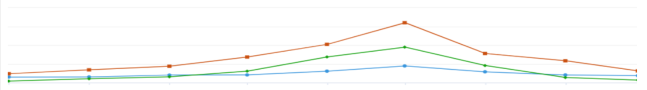
Legend:

• Red – Prophet only.
• Blue – ETS only.
• Green – Best fit.

Auto-ARIMA: The time traveler's delight

The auto-ARIMA algorithm is like a time machine. It takes you on a journey through past demand patterns so that you can make informed predictions about the future.

Auto-ARIMA uses a technique that is known as ARIMA. The name ARIMA is an abbreviation for the three key components that the technique combines:

• AR is short for "auto regressive." This component regresses the time series on its own previous values. It captures the influence of past values on the current value.
• I is short for "integrated." This component, which is also known as differencing, is a step that the model takes to morph a nonstationary time series into stationary data.
• MA is short for "moving average." This component accounts for past forecast errors and improves the model's accuracy by smoothing out the noise.

Therefore, the ARIMA technique combines autoregression and moving averages after it differences the data. The final prediction combines the influence of past values and the adjustments from past errors.

The auto-ARIMA algorithm automatically identifies the best combination of the three components to create a forecast model that suits your data. It follows these steps to generate forecasts:

1. Run differencing on the data if it isn't stationary.
2. Find correlation between lagged data points.
3. Calculate moving average error.

Auto-ARIMA works especially well with time series data that shows a stable pattern over time, such as seasonal fluctuations or trends. If your historical demand follows a reasonably consistent path, you might prefer to use auto-ARIMA as your forecasting method.

Auto-ARIMA algorithm equations

Auto regressive calculation

The AR component applies the following equation:

Y(t) = c + ɸ1Y(t−1) + ɸ2Y(t−2) + … + ɸpY(t−p) + ϵ(t)

Key:

• Y(t) – The value at time t.
• c – A constant.
• ɸ1, ɸ2, … ɸp – Coefficients of the model.
• ϵ(t) – The white noise error term.

Moving average calculation

The MA component applies the following equation:

Y(t) = c + ϵ(t) + ϴ1ϵ(t−1) + ϴ2ϵ(t−2) + … + ϴqϵ(t−q)

Key:

• Y(t) – The value at time t.
• c – A constant.
• ϵ(t), ϵ(t−1), … ϵ(t−q) – Error terms at time t, t−1, … t−q.
• ϴ1, ϴ2, … ϴq – Coefficients of the model.

ARIMA calculation

The auto-ARIMA algorithm combines the AR and MA components by using the following equation:

ARIMA = AR + MA (after differencing the time series)

ETS: The shape-shifter

ETS is a versatile demand forecasting algorithm that adapts to the shape of your data. It can change its approach based on the characteristics of your historical demand. Therefore, it's suitable for a wide range of scenarios.

The name ETS is an abbreviation for the three essential components that the algorithm decomposes the time series data into:

• E is short for "error." This component captures the random noise or irregular fluctuations.
• T is short for "trend." This component represents the overall direction of the data over time: increasing, decreasing, or constant.
• S is short for "seasonality." This component reflects repetitive patterns or cycles in the data (for example, yearly or monthly).

By understanding and modeling these components, ETS generates forecasts that capture the underlying patterns in your data.

ETS forecasts future data points by applying varying weights to different observations. More recent data points carry more weight than older ones. ETS can also decompose the time series into error, trend, and seasonality components. (The error comes from noise and fluctuations in the time series.) ETS uses the seasonal period parameter that the user sets as a seasonal index, estimates the trend in the upcoming horizon, and tries multiple values to determine what fits. Finally, it forecasts the error and combines it with the estimated trend and seasonality components.

Demand planning in Supply Chain Management determines which "flavor" of ETS is most suitable for each time series and applies it accordingly.

Here is a step-by-step explanation of the algorithm:

1. Decompose components. The time series is broken down into the three components: error (E), trend (T), and seasonality (S).

2. Select models for the components. Each component follows an additive model:

   ETS(A,A,A) – Additive error, additive trend, additive seasonality.

3. Specify the initial states. Initial values for the level, trend, and seasonality states of the model are calculated to start the recursive update process. The level is the baseline forecast, which is updated as the model is trained.

4. Update the states. As new data points arrive, the states of the model (level, trend, and seasonality) are updated by using weighted smoothing equations.

5. Forecast. Future values are predicted by combining the most recent estimates of the level, trend, and seasonality.

ETS algorithm equation

The ETS algorithm applies the following equation:

F(t+1) = αA(t) + [1−α]F(t)

Key:

• F(t+1) – The forecasted value.
• F(t) – The previous forecasted value.
• A(t) – The actual historical value.
• α – A smoothing constant (0 ≤ α ≤ 1).

Prophet: The visionary forecasting guru

Prophet was developed by Facebook's research team. It's a modern and flexible forecasting algorithm that can handle the challenges of real-world data. It's especially effective at handling missing values, outliers, and complex patterns. It performs best with seasonal data, accounts for holidays during forecasting, and doesn't need much preprocessing.

Prophet works by decomposing the time series data into several components, such as trend, seasonality, and holidays, and then fitting a model to each component. This approach enables Prophet to accurately capture the nuances in your data and produce reliable forecasts. Prophet is ideal for businesses that have irregular demand patterns or frequent outliers. It's also ideal for businesses that are affected by special events such as holidays or promotions.

The Prophet algorithm follows these steps to generate forecasts:

1. Decompose the time series into trend, seasonality, and holiday components.
2. Detect and handle change points for trend shifts.
3. Use Fourier series for seasonal patterns.
4. Add holiday regressors for irregular events.
5. Fit the model parameters by using Bayesian optimization.
6. Generate predictions and uncertainty intervals.

Prophet algorithm equation

The Prophet algorithm applies the following equation:

y(t) = g(t) + s(t) + h(t) + ϵ(t)

Key:

• g(t) – A value that captures the nonperiodic trend changes over time. It's calculated by using a piecewise linear trend equation.
• s(t) – A value that represents recurring seasonality patterns (for example, daily, weekly, or yearly). It's modeled by using Fourier series.
• h(t) – A value that accounts for known, irregular effects that are caused by holidays or special events. It treats these effects as additional regressors that allow for flexibility in the modeling of special events.
• ϵ(t) – Random noise or unexplained variability.

XGBoost

Unlike the other algorithms that this article describes, eXtreme Gradient Boosting (XGBoost) can generate a forecast based on two inputs. It's currently the only algorithm that you can use with the Forecast with signals forecast model step in Demand planning. In addition, it's supported only by that type of step. Learn more about how to set up forecast models that use XGBoost and signals input in Forecast with signals.

XGBoost is a highly efficient and scalable implementation of gradient boosting. It builds an ensemble of decision trees to make predictions. The following subsections break down each of the components.

Decision trees

A decision tree is a machine learning model that splits data into subsets based on signals values (also known as dimensions or features) and forms a tree-like structure. The following example shows sales based on weather data.

                          [Is temp > 25°C?]
                          /               \
                        Yes                No
                       /                     \
        [Is temp > 30°C?]               [Is temp > 15°C?]
            /      \                        /           \
         Yes        No                    Yes             No
         /            \                   /                \
    Leaf: 80      Leaf: 60        [Is temp > 10°C?]     Leaf: 20
                                        /       \
                                    Yes         No
                                    /            \
                                Leaf: 40      Leaf: 10

This decision tree progresses in the following way:

1. Root node – The tree splits based on whether the temperature exceeds 25°C:

   • Yes – Go to the left subtree.
   • No – Go to the right subtree.

2. Left subtree (temp > 25°C) – The tree further splits based on whether the temperature exceeds 30°C:

   • Yes – Predict 80 sales.
   • No – Predict 60 sales.

3. Right subtree (temp ≤ 25°C) – The tree splits based on whether the temperature exceeds 15°C:

   • Yes – The tree further splits based on whether the temperature exceeds 10°C:

     • Yes – Predict 40 sales.
     • No – Predict 10 sales.

   • No – Predict 20 sales.

Ensemble learning

Ensemble learning is a machine learning approach that combines multiple models (often referred to as weak learners) to make predictions. The idea is that the combined output of many models is often more accurate and robust than any single model.

One type of ensemble learning is known as boosting. In this approach, models are built sequentially, and each model corrects the errors of the previous one.

Gradient boosting

Gradient boosting is a powerful machine learning technique that is used for both regression (which is the case here) and classification problems. An ensemble of weak models (typically decision trees) is built sequentially, and each model focuses on reducing the errors (residuals) that the previous models made.

Gradient boosting is effective at capturing complex relationships between signals (also known as exogenous variables) and the input data (also known as the target variable). It also provides better predictive performance than other methods.

How the XGBoost algorithm works

XGBoost is a highly efficient and scalable implementation of gradient boosting. It builds an ensemble of decision trees to make predictions. Here is a step-by-step explanation of how it works:

1. Initialize predictions.

   • Task – Start by predicting a base value for all instances.
   • Purpose – The base value is typically the mean of the target variable for regression or the log odds for classification.

2. Calculate residuals (gradients).

   • Task – Compute the residuals or gradients, which represent the difference between the predicted and actual values.
   • Purpose – These residuals serve as the error signal that the model will try to minimize.

3. Fit a decision tree.

   • Task – Train a new decision tree by using the residuals (gradients) as the target values.

   • Purpose – The tree predicts adjustments to the previous model's predictions.

   • Key details

     • XGBoost uses a greedy algorithm to split the data.
     • Splits are selected based on the gain in the objective function, which is regularized to avoid overfitting.

4. Regularize tree growth.

   • Task – Apply constraints to prevent overfitting.

   • Purpose – Regularization helps generalize the model and maintain performance on unseen data.

   • Techniques

     • Tree depth – Limit the maximum depth of trees.
     • Leaf weights – Penalize overly complex trees by adding regularization terms.
     • Minimum split gain – Allow a split only if a minimum improvement occurs in the loss function.

5. Update predictions.

   • Task – Adjust predictions by adding the outputs of the new tree.
   • Purpose – This step reduces the error progressively.

6. Repeat the process.

   • Task – Repeat steps 2 through 5 to sequentially add more trees.

   • Purpose – Each tree reduces the residuals and therefore gradually improves the model.

   • Stopping criteria

     • A fixed number of trees are implemented in the algorithm of the Demand planning app.
     • There is no significant improvement in the loss function (convergence).

7. Combine trees for the final prediction.

   • Task – Aggregate the outputs of all trees to produce the final prediction.
   • Purpose – Each tree contributes to the final result. Therefore, an ensemble effect is created.

Custom Azure Machine Learning algorithm

If you have a custom Azure Machine Learning algorithm that you want to use with your forecasting models, you can use it in Demand planning.