Beispiele für bedingte Formatierung

Artikel
12/30/2023

Die bedingte Formatierung in Excel wendet die Formatierung auf Zellen basierend auf bestimmten Bedingungen oder Regeln an. Diese Formate werden automatisch angepasst, wenn sich die Daten ändern, sodass Ihr Skript nicht mehrmals ausgeführt werden muss. Diese Seite enthält eine Sammlung von Office-Skripts, die verschiedene Optionen für die bedingte Formatierung veranschaulichen.

Diese Beispielarbeitsmappe enthält Arbeitsblätter, die mit den Beispielskripts getestet werden können.

Herunterladen der Beispielarbeitsmappe

Zellwert

Die bedingte Formatierung von Zellenwerten wendet ein Format auf jede Zelle an, die einen Wert enthält, der einem bestimmten Kriterium entspricht. Dadurch können wichtige Datenpunkte schnell ermittelt werden.

Im folgenden Beispiel wird eine bedingte Zellwertformatierung auf einen Bereich angewendet. Bei jedem Wert unter 60 wird die Füllfarbe der Zelle geändert, und die Schriftart wird kursiv formatiert.

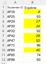
Eine Liste von Bewertungen mit jeder Zelle, die einen Wert unter 60 enthält, formatiert mit gelber Füllung und kursiv formatiertem Text.

function main(workbook: ExcelScript.Workbook) {
    // Get the range to format.
    const sheet = workbook.getWorksheet("CellValue");
    const ratingColumn = sheet.getRange("B2:B12");
    sheet.activate();
    
    // Add cell value conditional formatting.
    const cellValueConditionalFormatting =
        ratingColumn.addConditionalFormat(ExcelScript.ConditionalFormatType.cellValue).getCellValue();
    
    // Create the condition, in this case when the cell value is less than 60
    let rule: ExcelScript.ConditionalCellValueRule = {
        formula1: "60",
        operator: ExcelScript.ConditionalCellValueOperator.lessThan
    };
    cellValueConditionalFormatting.setRule(rule);
    
    // Set the format to apply when the condition is met.
    let format = cellValueConditionalFormatting.getFormat();
    format.getFill().setColor("yellow");
    format.getFont().setItalic(true);
}

Farbskala

Die bedingte Formatierung der Farbskala wendet einen Farbverlauf über einen Bereich an. Die Zellen mit den minimalen und maximalen Werten des Bereichs verwenden die angegebenen Farben, während andere Zellen proportional skaliert werden. Eine optionale Mittelpunktfarbe bietet mehr Kontrast.

Im folgenden Beispiel wird eine rote, weiße und blaue Farbskala auf den ausgewählten Bereich angewendet.

Eine Tabelle mit Temperaturen mit den niedrigeren Werten blau und den höheren Werten rot gefärbt.

function main(workbook: ExcelScript.Workbook) {
    // Get the range to format.
    const sheet = workbook.getWorksheet("ColorScale");
    const dataRange = sheet.getRange("B2:M13");
    sheet.activate();

    // Create a new conditional formatting object by adding one to the range.
    const conditionalFormatting = dataRange.addConditionalFormat(ExcelScript.ConditionalFormatType.colorScale);

    // Set the colors for the three parts of the scale: minimum, midpoint, and maximum.
    conditionalFormatting.getColorScale().setCriteria({
        minimum: {
            color: "#5A8AC6", /* A pale blue. */
            type: ExcelScript.ConditionalFormatColorCriterionType.lowestValue
        },
        midpoint: {
            color: "#FCFCFF", /* Slightly off-white. */
            formula: '=50', type: ExcelScript.ConditionalFormatColorCriterionType.percentile
        },
        maximum: {
            color: "#F8696B", /* A pale red. */
            type: ExcelScript.ConditionalFormatColorCriterionType.highestValue
        }
    });
}

Datenbalken

Die bedingte Formatierung von Datenbalken fügt einen teilweise gefüllten Balken im Hintergrund einer Zelle hinzu. Die Fülle des Balkens wird durch den Wert in der Zelle und den durch das Format angegebenen Bereich definiert.

Im folgenden Beispiel wird eine bedingte Datenbalkenformatierung für den ausgewählten Bereich erstellt. Die Skala des Datenbalkens reicht von 0 bis 1200.

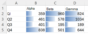
Eine Tabelle mit Werten mit Datenbalken, die ihren Wert im Vergleich zu 1200 anzeigen.


function main(workbook: ExcelScript.Workbook) {
    // Get the range to format.
    const sheet = workbook.getWorksheet("DataBar");
    const dataRange = sheet.getRange("B2:D5");
    sheet.activate();

    // Create new conditional formatting on the range.
    const format = dataRange.addConditionalFormat(ExcelScript.ConditionalFormatType.dataBar);
    const dataBarFormat = format.getDataBar();

    // Set the lower bound of the data bar formatting to be 0.
    const lowerBound: ExcelScript.ConditionalDataBarRule = {
        type: ExcelScript.ConditionalFormatRuleType.number,
        formula: "0"
    };
    dataBarFormat.setLowerBoundRule(lowerBound);

    // Set the upper bound of the data bar formatting to be 1200.
    const upperBound: ExcelScript.ConditionalDataBarRule = {
        type: ExcelScript.ConditionalFormatRuleType.number,
        formula: "1200"
    };
    dataBarFormat.setUpperBoundRule(upperBound);
}

Symbolsatz

Die bedingte Formatierung von Symbolen fügt jeder Zelle in einem Bereich Symbole hinzu. Die Symbole stammen aus einem angegebenen Satz. Symbole werden basierend auf einem geordneten Array von Kriterien angewendet, wobei jedes Kriterium einem einzelnen Symbol zugeordnet ist.

Im folgenden Beispiel wird die bedingte Formatierung des Symbols "Drei Ampel" auf einen Bereich angewendet.

function main(workbook: ExcelScript.Workbook) {
    // Get the range to format.
    const sheet = workbook.getWorksheet("IconSet");
    const dataRange = sheet.getRange("B2:B12");
    sheet.activate();

    // Create icon set conditional formatting on the range.
    const conditionalFormatting = dataRange.addConditionalFormat(ExcelScript.ConditionalFormatType.iconSet);

    // Use the "3 Traffic Lights (Unrimmed)" set.
    conditionalFormatting.getIconSet().setStyle(ExcelScript.IconSet.threeTrafficLights1);
    conditionalFormatting.getIconSet().setCriteria([
      { // Use the red light as the default for positive values.
        formula: '=0', operator: ExcelScript.ConditionalIconCriterionOperator.greaterThanOrEqual,
        type: ExcelScript.ConditionalFormatIconRuleType.number
      },
      { // The yellow light is applied to all values 6 and greater. The replaces the red light when applicable.
        formula: '=6', operator: ExcelScript.ConditionalIconCriterionOperator.greaterThanOrEqual,
        type: ExcelScript.ConditionalFormatIconRuleType.number
      },
      { // The green light is applied to all values 8 and greater. As with the yellow light, the icon is replaced when the new criteria is met.
        formula: '=8', operator: ExcelScript.ConditionalIconCriterionOperator.greaterThanOrEqual,
        type: ExcelScript.ConditionalFormatIconRuleType.number
      }
    ]);
}

Voreinstellung

Die voreingestellte bedingte Formatierung wendet ein angegebenes Format auf einen Bereich an, der auf gängigen Szenarien basiert, z. B. leere Zellen und doppelte Werte. Die vollständige Liste der voreingestellten Kriterien wird von der Enumeration ConditionalFormatPresetCriterion bereitgestellt.

Im folgenden Beispiel wird eine gelbe Füllung für eine leere Zelle im Bereich angezeigt.

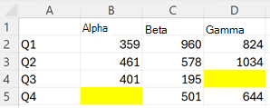
Eine Tabelle mit leeren Werten, die mit gelben Füllungen hervorgehoben sind.

function main(workbook: ExcelScript.Workbook) {
    // Get the range to format.
    const sheet = workbook.getWorksheet("Preset");
    const dataRange = sheet.getRange("B2:D5");
    sheet.activate();
    
    // Add new conditional formatting to that range.
    const conditionalFormat = dataRange.addConditionalFormat(
    ExcelScript.ConditionalFormatType.presetCriteria);
    
    // Set the conditional formatting to apply a yellow fill.
    const presetFormat = conditionalFormat.getPreset();
    presetFormat.getFormat().getFill().setColor("yellow");
    
    // Set a rule to apply the conditional format when cells are left blank.
    const blankRule: ExcelScript.ConditionalPresetCriteriaRule = {
        criterion: ExcelScript.ConditionalFormatPresetCriterion.blanks
    };
    presetFormat.setRule(blankRule);
}

Textvergleich

Die bedingte Formatierung von Textvergleichen formatiert Zellen basierend auf ihrem Textinhalt. Die Formatierung wird angewendet, wenn der Text mit beginnt, enthält, endet mit oder enthält die angegebene Teilzeichenfolge nicht.

Im folgenden Beispiel wird jede Zelle im Bereich markiert, die den Text "Überprüfen" enthält.

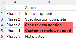
Eine Tabelle mit status Einträgen, in denen jede Zelle, die das Wort

function main(workbook: ExcelScript.Workbook) {
    // Get the range to format.
    const sheet = workbook.getWorksheet("TextComparison");
    const dataRange = sheet.getRange("B2:B6");
    sheet.activate();

    // Add conditional formatting based on the text in the cells.
    const textConditionFormat = dataRange.addConditionalFormat(
        ExcelScript.ConditionalFormatType.containsText).getTextComparison();

    // Set the conditional format to provide a light red fill and make the font bold.
    textConditionFormat.getFormat().getFill().setColor("#F8696B");
    textConditionFormat.getFormat().getFont().setBold(true);

    // Apply the condition rule that the text contains with "review".
    const textRule: ExcelScript.ConditionalTextComparisonRule = {
        operator: ExcelScript.ConditionalTextOperator.contains,
        text: "review"
    };
    textConditionFormat.setRule(textRule);
}

Oben/unten

Die bedingte Formatierung oben/unten markiert die höchsten oder niedrigsten Werte in einem Bereich. Die Hochs und Tiefen basieren entweder auf Rohwerten oder Prozentsätzen.

Im folgenden Beispiel wird eine bedingte Formatierung angewendet, um die beiden höchsten Zahlen im Bereich anzuzeigen.

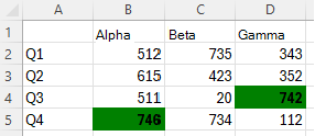
Eine Verkaufstabelle, in der die beiden obersten Werte mit einer grünen Füllung und einer fett formatierten Schriftart hervorgehoben sind.

function main(workbook: ExcelScript.Workbook) {
  // Get the range to format.
  const sheet = workbook.getWorksheet("TopBottom");
  const dataRange = sheet.getRange("B2:D5");
  sheet.activate();

    // Set the fill color to green and the font to bold for the top 2 values in the range.
    const topBottomFormat = dataRange.addConditionalFormat(ExcelScript.ConditionalFormatType.topBottom).getTopBottom();
    topBottomFormat.getFormat().getFill().setColor("green");
    topBottomFormat.getFormat().getFont().setBold(true);
    topBottomFormat.setRule({
      rank: 2, /* The numeric threshold. */
      type: ExcelScript.ConditionalTopBottomCriterionType.topItems /* The type of the top/bottom condition. */
    });
}

Benutzerdefinierte Bedingungen

Mit der benutzerdefinierten bedingten Formatierung können komplexe Formeln definieren, wann die Formatierung angewendet wird. Verwenden Sie diese Option, wenn die anderen Optionen nicht ausreichen.

Im folgenden Beispiel wird eine benutzerdefinierte bedingte Formatierung für den ausgewählten Bereich festgelegt. Eine hellgrüne Füllung und fett formatierte Schriftart werden auf eine Zelle angewendet, wenn der Wert größer als der Wert in der vorherigen Spalte der Zeile ist.

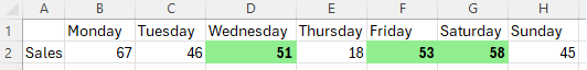
Eine Zeile einer Sales-Tabelle. Werte, die höher als der linke wert sind, weisen eine grüne Füllung und eine fett formatierte Schriftart auf.

function main(workbook: ExcelScript.Workbook) {
    // Get the range to format.
    const sheet = workbook.getWorksheet("Custom");
    const dataRange = sheet.getRange("B2:H2");
    sheet.activate();
    
    // Apply a rule for positive change from the previous column.
    const positiveChange = dataRange.addConditionalFormat(ExcelScript.ConditionalFormatType.custom).getCustom();
    positiveChange.getFormat().getFill().setColor("lightgreen");
    positiveChange.getFormat().getFont().setBold(true);
    positiveChange.getRule().setFormula(
        `=${dataRange.getCell(0, 0).getAddress()}>${dataRange.getOffsetRange(0, -1).getCell(0, 0).getAddress()}`
    );
}

Freigeben über