Microsoft’s software for quantum computing, Liqui|>

Guest post by Vani Asawa Microsoft Student Partner at Oxford University

About me

Hi! I am Vani Asawa, a second year student at the University of Oxford studying Mathematics. Originally from India. I have always been very passionate about science and technology and knew from a very young age that I would be working in those areas. I am particularly interested in understanding the applications of Machine Learning and Big Data. At Oxford, I am involved with the Artificial Intelligence Society as the Social Media Director, working to make my peers realise the potential of Artificial Intelligence and organising events with speakers working in this field.

Introduction

Alan Turing invented the programmable computer in 1936 to show that certain mathematical problems could not be solved computationally. He believed that a computer, armed with the necessary resources, is capable of realizing any reasonable algorithm.

Since then, the computer industry has not only managed to build programmable computing machines, but also managed to double their capabilities every few months. However, despite these advances in computer technology, modern computers are still unable to make significant dents in hard problems. Problems that require exponential resources remain as intractable today as they were in 1936.

Enter Quantum Computing

With its ability to harness quantum-mechanical phenomenon such as superposition and entangling, quantum computing uses the power of atoms to perform memory and processing tasks. In just hours or days, a quantum computer can solve complex problems that would otherwise take years for a traditional computer to solve. This will have massive implications for research in energy, medicine, artificial intelligence, environmental systems, smart materials, investments, logistics and supply chains, and more.

Through this blog, you will not only be able to find out more about the power of quantum computing and its impact on our future economy, but also be able to start building quantum applications using Microsoft’s software for quantum computing, Liqui|>!

Let’s get started!

What is Quantum Computing?

“Quantum Computing” is the use of quantum mechanical systems with the full use of their quantum mechanical properties to do computations.

What does this mean?

Think of a modern, or classical computer. Classical computers store information in bits. Equivalent to an atom, a bit is the smallest unit of information storage. Each bit can take the value of 1 or 0. These 1s and 0s act as on/off switches that ultimately drive computer operations.

Quantum computers, on the other hand, are based on qubits, which operate according to two key principles of quantum physics: superposition and entanglement.

- By the principles of superposition, each qubit can represent both a 1 and a 0 at the same time.

- As a result of entanglement, the state of a qubit, or the property of a qubit being 1 or 0, can depend on the state of another qubit being 1 or 0.

Using these two principles, qubits can act as more sophisticated switches, enabling quantum computers to function in ways that allow them to solve difficult problems that are intractable using today’s computers.

Pictorially, a qubit can be thought of as follows:

Whereas a classical bit can only be in two states - in this case, the two poles of the sphere |0> and |1>, a qubit can be any complex vector form the centre of the sphere pointing to a spot on the unit sphere.

Thus, unlike classical bits, qubits arise in the way that they can simultaneously exist as both 0 and 1, with the probability for each state given by a numerical coefficient. Describing a two- qubit quantum computer thus requires four coefficients. Generalising for an n-qubit quantum system, we observe that n qubits demand 2ⁿnumbers, which rapidly becomes a sizable set for larger values of n. For example, if n equals 100, about 10³⁰ numbers are required to describe all the probabilities for all the possible states of the quantum machine—a number that exceeds the capacity of the largest conventional computer. Thus, a quantum computer could naturally perform myriad operations simultaneously, or in parallel, using only a single processing unit.

Now that we have understood the ideology behind quantum computing, let’s take a look at what is LIQ|⟩ and some key terminologies before we get started on coding quantum application!

LIQ|⟩

LIQ|⟩, or “Language-Integrated Quantum Operations”, is a software for developing quantum applications. Currently being developed by the Quantum Architectures and Computation Group (QuArC) at Microsoft Research, LIQ|⟩ includes a programming language, optimization and scheduling algorithms, and quantum simulators to aid in the development and understanding of quantum protocols, quantum algorithms, quantum error correction, and quantum devices.

Currently, there are three classes of simulators built into the system representing different levels of abstraction:

1. Physical Modeling: One of the slowest simulators by nature, the physical modelling simulator attempts to model some of the actual physics in a quantum system.

2. Universal Modeling: This simulator is highly optimized for performing multiple calculations simultaneously, and is highly efficient in memory usage. However, its main limitation is the number of qubits (~30) that can be entangled at one time.

3. Stabilizer Modeling: This simulator has the virtue of allowing large circuits on tens of thousands of qubits, but has limitations on the types of operations.

These Simulations can be accomplished in the following ways:

1. Test Mode: Functions that are built into the software can be called from the command line prompt and run.
2. Script Mode: The system can be run directly from an F# text file. There is no separate language compilation required, and the entire simulation can be available from this mode.
3. Function Mode : This mode involves a compilation environment and the use of a .Net language, typically F#. The user is free to build their own application using the APIs available in the F# environment.
4. Circuit Mode : Function mode can be compiled into a circuit data structure, which can be manipulated by the user in several ways, such as running through built-in optimizers, having quantum error correction added, and exporting for use in other environments.

Some other key terminologies that will be useful to know before we learn how to code quantum applications are:

1. Ket refers to the complete state of the system, and is of the length 2ⁿ where n is the number of qubits in the state.
2. Gate refers to a matrix that is used to represent an operation, such as measurement and reanimation, that can be applied to a set of qubits.
3. Finally, Circuits are used to represent a list of operations on gates. They can provide pre-processing of quantum algorithms for various reasons, such as performing multiple operations (or parallelizing) , substitution (some gates will not be available in target physical systems), and optimization.

Why LIQ| ⟩ ?

LIQUi| ⟩ allows the simulation of Hamiltonians, quantum circuits, quantum stabilizer circuits, and quantum noise models, and supports Client, Service, and Cloud operation. It allows the user to express circuits in a high-level functional language like F#, and supports the extraction of circuit data structures that can be passed to other components for circuit optimization, quantum error correction or gate replacement.

As a user, you can use LIQUi| ⟩ to define quantum circuits, render them into a variety of graphical formats, and execute them using an appropriate simulator. Some of the specific algorithms you can simulate with LIQUi| ⟩ are:

● Simple quantum teleportation

● Shor’s factoring algorithm

● Quantum chemistry: computing the ground state energy of a molecule

● Quantum error correction

Getting Started

Depending on your platform of choice, following are the steps for installing LIQUi| ⟩ :

WINDOWS

1. Install Visual Studio: Download the official MSI Installer. This will install the tools and put them on your PATH. Make sure you select F# as one of the languages to install.

03/01/2016 10:14 AM <DIR> .

03/01/2016 10:14 AM <DIR> ..

03/01/2016 10:14 AM 10,086 AzureGuide.md

03/01/2016 10:14 AM <DIR> bin

03/01/2016 10:14 AM <DIR> docs

03/01/2016 10:14 AM 17,292 GettingStarted.md

03/01/2016 10:14 AM <DIR> img

03/01/2016 10:14 AM 6,118 LICENSE.md

03/01/2016 10:14 AM <DIR> linux

03/01/2016 10:14 AM 32,708 LiquidTikZ.tex

03/01/2016 10:14 AM 5,441 README.md

03/01/2016 10:14 AM <DIR> Samples

03/01/2016 10:14 AM <DIR> source

03/01/2016 10:14 AM <DIR> UserCode

5 File(s) 71,645 bytes

1. 2. Install LIQUi| ⟩ : Download the zip file from GitHub. Extract the contents into C:\. This will create C:\Liquid-master - rename the directory to C:\Liquid.
   3. Run the App: Go into the C:\Liquid\bin directory, run the app and accept the license!

0:0000.0/===================================================================================================

0:0000.0/= The Language-Integrated Quantum Operations (LIQUi|>) Simulator =

0:0000.0/= is made available under license by Microsoft Corporation =

0:0000.0/= License terms may be viewed at https://github.com/msr-quarc/Liquid/blob/master/LICENSE.md =

0:0000.0/= Please type Y, followed by return, to indicate your acceptance of these terms =

0:0000.0/===================================================================================================

Y

UBUNTU (14.04)

1. Install Mono and F# - Make sure you remove any previous installations of the two to avoid incompatibilities!

$ sudo apt-key adv --keyserver keyserver.ubuntu.com --recv-keys 3FA7E0328081BFF6A14DA29AA6A19B38D3D831EF

$ echo "deb https://download.mono-project.com/repo/debian wheezy main" |

sudo tee /etc/apt/sources.list.d/mono-xamarin.list

$ sudo apt-get update

$ sudo apt-get install mono-complete fsharp

2. 2. Install LIQUi| ⟩ : Download the zip file from GitHub. Extract the contents into your home directory. This will create ~/Liquid-master - copy to the final destination

$ cd ~/Liquid-Master

$ sudo mkdir /Liquid

$ sudo chown $USER /Liquid

$ cp * /Liquid --recursive

2. 3. Run the app: Go into the /Liquid/linux directory, run the app and accept the license.

0:0000.0/===================================================================================================

0:0000.0/= The Language-Integrated Quantum Operations (LIQUi|>) Simulator =

0:0000.0/= is made available under license by Microsoft Corporation =

0:0000.0/= License terms may be viewed at https://github.com/msr-quarc/Liquid/blob/master/LICENSE.md =

0:0000.0/= Please type Y, followed by return, to indicate your acceptance of these terms =

0:0000.0/===================================================================================================

Y

OSX (10.11)

1. Install Mono and F#: https://www.mono-project.com/download/
2. Install LIQ⏐〉
   1. Download the zip file from GitHub.
   2. From your Downloads, open the folder Liquid-master.
   3. Select and Copy all the files..
   4. Type Shift-Command-G and then a slash (/) to go to the root.
   5. Type Shift-Command-N to create a new folder, and create the Liquid folder.
   6. Double click on the Liquid folder paste the contents of the downloaded Liquid-master tree into \Liquid.
3. Run the app: Go into the /Liquid/linux directory, run the app and accept the license

Vani:~ vaniasawa$ cd /Liquid/linux

Vani:linux vaniasawa$ mono Liquid.exe

0:0000.0/===================================================================================================

0:0000.0/= The Language-Integrated Quantum Operations (LIQUi|>) Simulator =

0:0000.0/= is made available under license by Microsoft Corporation =

0:0000.0/= License terms may be viewed at https://github.com/msr-quarc/Liquid/blob/master/LICENSE.md =

0:0000.0/= Please type Y, followed by return, to indicate your acceptance of these terms =

0:0000.0/===================================================================================================

Y

0:0000.5/===================================================================================================

0:0000.5/= Thank you for accepting the license terms =

0:0000.0/===================================================================================================

Y

Example of a Quantum Application - Spin Glass Simulation

Spin Glass - An Introduction

The study of spin glasses was inspired by the known physics of structural glasses (like window glass). Typical solid phases have crystalline ground states, where the atoms are arranged in a simple periodic arrangement, but window glass has amorphous arrangements of atoms. Now, to form glass, you need to quench the molten glass, so that it cools very rapidly and does not have time to "find" its crystalline ground state. Once it is at room temperature, it is so cold that the probability of the atoms in the glass finding their crystalline ground state, which is suppressed by a factor of e^−ϵ/T for some energy barrier ϵ, is negligibly small.

Now, just as the atoms in the glass are trapped in local minima of the energy, but globally the glass is not in its ground state, physicists noted that the same thing could happen in simple models of magnetism. Suppose that you have a magnet whose Hamiltonian energy is given by

H=∑_ij J_ij s_i s_j

where s_i ∈ {+1,−1}, and the couplings J_ij between various spins look random: sometimes positive, and sometimes negative. In general, this system will be frustrated: some of the bonds will have "unfavorable" energies: e.g., a positive J_ij with s_i=s_j. However, there certainly exists a ground state for the magnet and it is quite likely that some bonds will be frustrated, but the idea is that the existence of frustration typically leads to a very large number of local minima in the energy H, just as there are many local minima in a window glass.

So how do we define what a spin glass is? A heuristic physicist's definition of a spin glass is as follows:

A spin glass should have two properties:

1) An exponential number of locally stable equilibria, which do not have to be Hamiltonian

2) If you give the system reasonable dynamical rules, there are dynamics on all time scales. The simple way to see that this will happen is to recognize that the local minima in your system consist of clusters of spins of very large size, which all have to simultaneously flip, to get from one ground state to another. This cluster can be taken to be connected without loss of generality. Dynamics on all time scales then, heuristically, maps to the presence of clusters of all sizes. This leads to aging, where the system takes a very long time to relax to its ground state. In many models, aging breaks ergodicity -- the system will never explore the full phase space, but is trapped in some very small pocket of it.

Spin Glass Simulation

The Spin class in LIQ⏐〉 is used to define Spin-Glass problems to the system. The Hamiltonian being simulated is:

=Γ(t)∑_i Δ_ii+Λ(t)( ∑_ih_ii+∑ _{i<j ij ii} )

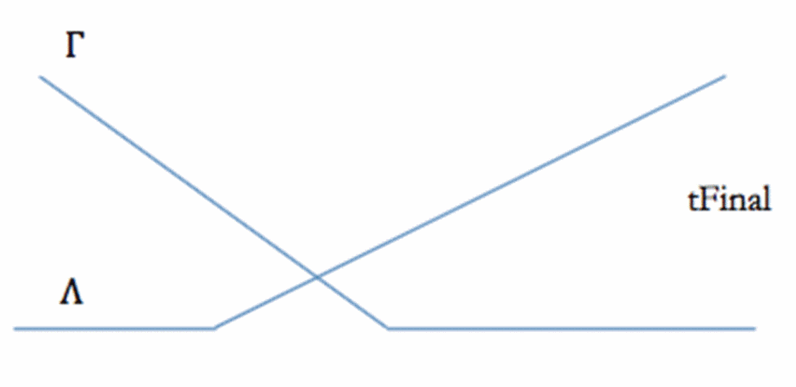
We are starting in a ground state that we know in the direction (Γ = 1, Λ = 0 ) and ending in a target state in the direction (when Γ = 0, Λ = 1) which we’d like to discover. This is referred to as an adiabatic evolution since it is expected that if we move slowly enough (changing Γ, Λ) we can stay in the ground state of the entire system and smoothly move to the solution. The changing of strength over time is called the annealing schedule and typically looks like this:

There are two main ways to instantiate the class. The first is the “bottom level” version that lets you specify everything:

type Spin(
spinTerms : SpinTerm list,
numSpins : int,
runMode : RunMode)

The constructor arguments are:

1. spinTerms which are a list of elements that contain:

a. schedule:0 based index of an annealing schedule that will be used

b. op: Operation(Gate) to apply

c. ampl: Amplitude(strength) of this term

2. numSpins: How many spins are there(qubits)

3. runMode:Trotterization to use:

a. Trotter1: First order Trotter term

b. Trotter1x: Split the transvers (X) field terms to the start and end of the Circuit

c. Trotter2: Second order Trotterization

The second form of the constructor takes care of many of the details for you:

type Spin(
hs : Dictionary<int,float>,
Js : Dictionary<int*int,float>)

The constructor arguments are:

● hs – Create a dictionary for each Qubits that you want to provide a strength to in the range (typically) of -1.0 to +1.0. These are the ZR terms.

● Js – Coupling strength between two Qubits. This is a dictionary of Qubit Id pairs and strength. Only Ids where the first is less than the second is searched for (i<j) and typical values are -1.0 which is ferromagnetic coupling and +1.0 which is antiferromagnetic coupling (0.0 = no coupling). These are the ZZR terms.

Note that there’s no XR term, since it’s implied automatically and is on annealing schedule 0. The ZR and ZZR are terms on automatically placed on schedule 1.

Two built-in static members are available to aid in setting up spin-glass systems. Let’s go through the example provided in the samples directory (Ferro.fsx) which simulates a ferromagnetic chain. The file shows both static members, but take a look at the simpler one here:

let tests = 50 // Tests to run
let qCnt = 12 // Qubit count
let h0 = 1.0 // h0: Left most qubit Z strength
let hn = -1.0 // hn: Right most qubit z strength
let coupling= 1.0 // 1=ferro -1=anti-ferro 0=none
let sched = [(100,0.0,1.0)] // Annealing schedule
let runonce = true // Runonce: Virtual measurements

let decohere= [] // No decoherence model

Spin.Ferro(tests,qCnt,h0,hn,coupling,sched,runonce,decohere)

The arguments are:

1. tests: How many instances to run.
2. qCnt: Total number of qubits to use as spin terms
3. h0: Strength of the h term on Qubit 0. +1 = Force spin up
4. hn: Strength of the h term on the last Qubit. -1 = Force spin down
5. coupling:Strengthofthebetweenqubitterms(buildaferromagneticchain by specifying +1.0)
6. sched: At time 0, schedule 0 is always 1.0 (the term) and all the other schedules are at 0.0 . For this reason, we only need to specify the ending point for the schedules. Here we’ve specified a final time of 100 where the term (schedule 0) becomes 0.0 and the terms (schedule 1) become 1.0.
7. runonce: This is a simulation optimization that lets us run a test once and then look directly into the state vector (since we’re a simulator) and obtain all the probabilities instead of running 100s or 1000s of times and measuring to get the same result (which we’d have to actually do on a quantum computer).
8. decohere: This is an advanced option that allows dechoherence models to be plugged in. For this test, we’re using perfect qubits.

What we’ve done is created a twisted chain (one end up; one end down) so when we simulate, we get both details for 1 run and a histogram across all runs:

0:0000.0/ 1%: ............ [<H>=-6.000 Stdev 0.000] [S_mid=0.000]

0:0000.0/ 10%: -..........+ [<H>=-5.525 Stdev 0.043] [S_mid=0.009]

0:0000.0/ 18%: 0..........1 [<H>=-5.242 Stdev 0.049] [S_mid=0.036]

0:0000.0/ 20%: 0-........+1 [<H>=-5.197 Stdev 0.049] [S_mid=0.048]

0:0000.0/ 25%: 0--......++1 [<H>=-5.142 Stdev 0.058] [S_mid=0.095]

0:0000.0/ 26%: 00-......+11 [<H>=-5.142 Stdev 0.061] [S_mid=0.108]

0:0000.0/ 28%: 00--....++11 [<H>=-5.154 Stdev 0.065] [S_mid=0.139]

0:0000.0/ 30%: 000-....+111 [<H>=-5.185 Stdev 0.069] [S_mid=0.180]

0:0000.0/ 32%: 000--..++111 [<H>=-5.234 Stdev 0.070] [S_mid=0.228]

0:0000.0/ 34%: 0000-..+1111 [<H>=-5.303 Stdev 0.067] [S_mid=0.267]

0:0000.0/ 81%: 00000..11111 [<H>=-9.031 Stdev 0.060] [S_mid=0.631]

0:0000.1/!Histogram:

0:0000.1/!Ferro 6.0% 000000000001 (E=-11.0000) [ones= 1]

0:0000.1/!Ferro 10.0% 000000000011 (E=-11.0000) [ones= 2]

0:0000.1/!Ferro 8.0% 000000000111 (E=-11.0000) [ones= 3]

0:0000.1/!Ferro 12.0% 000000001111 (E=-11.0000) [ones= 4]

0:0000.1/!Ferro 4.0% 000000011111 (E=-11.0000) [ones= 5]

0:0000.1/!Ferro 12.0% 000000111111 (E=-11.0000) [ones= 6]

0:0000.1/!Ferro 30.0% 000001111111 (E=-11.0000) [ones= 7]

0:0000.1/!Ferro 6.0% 000011111111 (E=-11.0000) [ones= 8]

0:0000.1/!Ferro 2.0% 000111111111 (E=-11.0000) [ones= 9]

0:0000.1/!Ferro 10.0% 001111111111 (E=-11.0000) [ones=10]

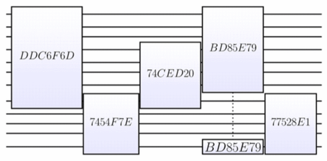
The detailed output shows the probability of each qubit between 0 and 1 (- = tending to 0, +=tending to 1 and .= no tendency). The histogram shows each case seen, what percentage of the runs fell into that category and the final energy (showing we reached the ground state). The test also generated two diagrams. The first was Ferro.htm which shows all the pieces (as well as the fact that we used RunMode Trotter1X visible from the fact that the RpX gates are both at the beginning and end of the Circuit):

The second diagram shows the Circuit that was actually run after “Gate Growing” was performed:

 

Here you can see that we only had to do 5 matrix multiplies to perform the entire circuit (major speed-up). One of the reasons not to grow even further is that the circuit changes at every time step (due to the annealing schedule), so spending time optimizing beyond a certain point simply doesn’t pay.

The Spin.Test(...) static routine allows arbitrary connections (not just chains) and much finer control (including Trotter number).

Conclusion

Today, quantum computing is somewhere between the arrival of FORTRAN and Engelbart’s “Mother of all Demos.” Highly trained specialists are able to translate real world problems into language a quantum computer can understand, but for most people the technology is out of reach. That will change in the years to come.

It might not be that we have quantum computers in all our homes, but we will likely be able to access them in the cloud and they will help us solve problems that seem impossible today. According to D-Wave’s Jeremy Hilton,“the quantum computing revolution may be even more profound than the digital computing revolution a half century ago and it will happen much faster.”

Excited? Want to find out more about Quantum Applications?

Take a look at the following links and go explore the world of quantum applications and LIQ⏐〉!

https://github.com/StationQ/Liquid  https://msr-quarc.github.io/Liquid/LIQUiD.pdf https://www.microsoft.com/en-us/quantum/default.aspx https://www.microsoft.com/en-us/research/project/language-integrated-quantum-operations-liqui/ https://cdn.nanalyze.com/uploads/2017/04/Dilbert-Quatum-Computing.gif https://www.quora.com/What-is-a-spin-glass-and-how-did-the-study-of-spin-glasses-get-started https://www.forbes.com/sites/gregsatell/2016/10/02/heres-how-quantum-computing-will-change-the-world/#30d053c0ad6d

Comments

• Anonymous
  December 27, 2017
  Thank you!