An approach to breaking loop carried dependencies - Parallel Wavefront
Loop-carried dependencies are dependencies where one iteration of the loop depends upon the results of another iteration of the loop
Question: How do I parallelize for-loops with no loop carried dependencies?
Answer: There is an excellent blog on parallel_for by Marko, one of our senior developers in the team, that addresses the question above.
Question: How do I parallelize for-loops with loop carried dependencies?
Answer: It depends (on the dependencies)!!
As cryptic as the answer is, it really comes down to modeling the dependencies and usually altering the algorithm to break loop carried dependencies. Sometimes this might be possible, other times, it may not be feasible, perhaps because of performance and/or because of the effort involved in parallelizing the approach.
Lets dive down a little deeper into this with an example. Consider the following dynamic programming algorithm that uses the Smith-Waterman approach to align 2 biological sequences. At a high-level, the Smith-Waterman approach for aligning two biological sequences a and b consists of the following two main steps:
1) Populating a m x n matrix, thereby finding the winning node that corresponds to a row & column
2) Backtracking from the winning node, to find optimal alignment
The edges (row=0's and col=0's) have predefined value (=0). We calculate score of every node based on the maximum values of:
i) Local alignment (match/mismatch) score : dependent on diagonal max local align score + similarity/mismatch score from ScoringMatrix(H(i-1, j-1) + SimilarityScore(A[i], B[j]))
ii) Deletion score (dependent on left cell's deletion and score values)
iii) Insertion score (dependent on top cell's insertion and score values)
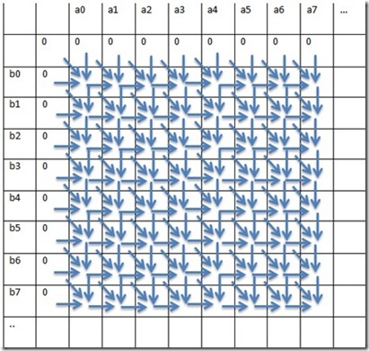
To simplify, every element[i, j] in the matrix has dependencies on [i, j-1], [i-1, j-1] and [i-1, j] values
Fig 1. Depiction of dependencies in the matrix
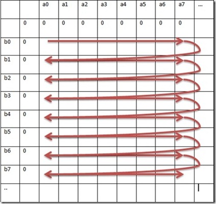
When parsing the matrix serially, the most trivial approach is to have two loops (1 based on query length and 1 based on subject length).
Pseudo-code for the serial approach is given below:
For (row=1..subjectlength)
For(col=1..querylength)
hVal = similarity(row, col) + blosum62(row,col)
eVal[row][col] = max(eVal[row-1][col]-gapExtn, score[row-1][col]-gapOpen)
fVal[row][col] = max(fVal[row][col-1]-gapExtn, score [row][col-1]-gapOpen)
score [row][col] = max(hVal, eVal[row][col],fVal[row][col], 0)
traceback[row][col] = winner(hVal, eVal[row][col],fVal[row][col], 0)
maxscore=max(maxscore, score [row][col])
EndFor
EndFor
Fig 2. Serial approach
To give you an idea of what it looks like in C++ (code snippet):
    1: Element Populate(int gap_open, int gap_extn)
    2: {
    3:     Element elem;
    4:     int row, col, localAlignScore_F, diagonalMaxLocalAlignScore_H, localAlignScore_H;
    5:
    6:     for (row = 1; row < m_subjectLength; ++row)
    7:     {
    8:         localAlignScore_F = 0;
    9:         diagonalMaxLocalAlignScore_H = m_pMaxLocalAlignScore_H[0];
   10:
   11:         for (col = 1; col < m_queryLength; ++col)
   12:         {
   13:             //Calc local alignment (match/mismatch) score: H(i-1, j-1) + SimilarityScore(A[i], B[j])
   14:             localAlignScore_H = diagonalMaxLocalAlignScore_H + m_matrix.GetScore(m_pSubject[row-1], m_pQuery[col-1]);
   15:
   16:             //Calc deletion score
   17:             m_pLocalAlignScore_E[col] = max((m_pLocalAlignScore_E[col] - gap_extn), (m_pMaxLocalAlignScore_H[col] - gap_open));
   18:
   19:             //Calc insertion score
   20:             localAlignScore_F = max((localAlignScore_F - gap_extn), (m_pMaxLocalAlignScore_H[col - 1] - gap_open));
   21:
   22:             //Store away the diag score
   23:             diagonalMaxLocalAlignScore_H = m_pMaxLocalAlignScore_H[col];
   24:
   25:             //Calculate matrix value h(i,j) = max{(h(i-1, j-1) + Z[A[i], B[j]]), e(i,j), f(i,j), 0}
   26:             m_pMaxLocalAlignScore_H[col] = MAX4(localAlignScore_H, m_pLocalAlignScore_E[col], localAlignScore_F, 0);
   27:
   28:             // Determine the traceback direction
   29:             (m_pMaxLocalAlignScore_H[col] == localAlignScore_H) ? m_ppDirectionMatrix[row][col] += DIAG : __noop;
   30:             (m_pMaxLocalAlignScore_H[col] == m_pLocalAlignScore_E[col]) ? m_ppDirectionMatrix[row][col] += TOP: __noop;
   31:             (m_pMaxLocalAlignScore_H[col] == localAlignScore_F) ? m_ppDirectionMatrix[row][col] += LEFT : __noop;
   32:
   33:             // Set the traceback start at the current elem i, j and score
   34:             (m_pMaxLocalAlignScore_H[col] > elem.GetScore()) ? elem.Set(row, col, m_pMaxLocalAlignScore_H[col]) : __noop;
   35:         }
   36:     }
   37:     return elem;
   38: }
Parallel Wavefront:
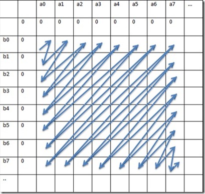
For effectively parallelizing the inner loop, we need to ensure that there are no loop-dependencies within the iterations of the inner loops (iterations of the outer loop may be dependent on its previous iterations and that's ok since we are not parallelizing the outer loop). We achieve this by calculating diagonals.
Caveat: Parallelizing loops that are too fine grained or consume a lot of bandwidth is a documented anti-pattern and contribute negatively to overall performance and/or scaling.
Fig 3. Parallel Wavefront approach
    1: Element Populate(int gap_open, int gap_extn)
    2: {
    3:     Element elem;
    4:
    5:     int iter=1, iterLength=1;
    6:     volatile LONG row, col;
    7:     bool fContinue = true;
    8:     int minVal = min(m_subjectLength, m_queryLength);
    9:     int maxVal = max(m_subjectLength, m_queryLength);
   10:     critical_section cslock;
   11:
   12:     auto Align = [&] (int loopCtr)
   13:     {
   14:         const int thisRow = row - loopCtr;
   15:         const int thisCol = col + loopCtr;
   16:
   17:         assert((thisRow > 0) && (thisRow < m_subjectLength));
   18:         assert((thisCol > 0) && (thisCol < m_queryLength));
   19:
   20:         //Calc local alignment (match/mismatch) score: H(i-1, j-1) + SimilarityScore(A[i], B[j])
   21:         const int localAlignScore_H = m_ppScoreMatrix[thisRow-1][thisCol-1].m_maxScore + m_matrix.GetScore(m_pSubject[thisRow-1], m_pQuery[thisCol-1]);
   22:
   23:         //Calc deletion score
   24:         m_ppScoreMatrix[thisRow][thisCol].m_localAlignScore_E = max((m_ppScoreMatrix[thisRow-1][thisCol].m_localAlignScore_E - gap_extn), (m_ppScoreMatrix[thisRow-1][thisCol].m_maxScore - gap_open));
   25:
   26:         //Calc insertion score
   27:         m_ppScoreMatrix[thisRow][thisCol].m_localAlignScore_F = max((m_ppScoreMatrix[thisRow][thisCol-1].m_localAlignScore_F - gap_extn), (m_ppScoreMatrix[thisRow][thisCol-1].m_maxScore - gap_open));
   28:
   29:         //Calculate matrix value h(i,j) = max{(h(i-1, j-1) + Z[A[i], B[j]]), e(i,j), f(i,j), 0}
   30:         m_ppScoreMatrix[thisRow][thisCol].m_maxScore = MAX4(localAlignScore_H, m_ppScoreMatrix[thisRow][thisCol].m_localAlignScore_E, m_ppScoreMatrix[thisRow][thisCol].m_localAlignScore_F, 0);
   31:
   32:         // Determine the traceback direction
   33:         ( m_ppScoreMatrix[thisRow][thisCol].m_maxScore == localAlignScore_H) ? m_ppScoreMatrix[thisRow][thisCol].m_direction += DIAG : __noop;
   34:         ( m_ppScoreMatrix[thisRow][thisCol].m_maxScore == m_ppScoreMatrix[thisRow][thisCol].m_localAlignScore_E) ? m_ppScoreMatrix[thisRow][thisCol].m_direction += TOP: __noop;
   35:         ( m_ppScoreMatrix[thisRow][thisCol].m_maxScore == m_ppScoreMatrix[thisRow][thisCol].m_localAlignScore_F) ? m_ppScoreMatrix[thisRow][thisCol].m_direction += LEFT : __noop;
   36:
   37:         // Set the traceback start at the current elem i, j and score
   38:         if (m_ppScoreMatrix[thisRow][thisCol].m_maxScore > elem.GetScore())
   39:         {
   40:             critical_section::scoped_lock slock(cslock);
   41:             (m_ppScoreMatrix[thisRow][thisCol].m_maxScore > elem.GetScore()) ? elem.Set(thisRow, thisCol, m_ppScoreMatrix[thisRow][thisCol].m_maxScore) : __noop;
   42:         }
   43:     };
   44:
   45:     while(fContinue)
   46:     {
   47:         //Decide row, col
   48:         row = min(iter, m_subjectLength-1);
   49:         (iter > m_subjectLength-1) ? col = (iter - m_subjectLength + 2) : col = 1;
   50:
   51:         //Calculate iteration length
   52:         if (iter  < minVal-1)
   53:         {
   54:             iterLength = iter;
   55:         }
   56:         else if (iter >= maxVal-1)
   57:         {
   58:             iterLength = minVal - (iter - maxVal) - 2;
   59:             (iterLength == 1) ? fContinue = false : __noop;
   60:         }
   61:         else
   62:         {
   63:             iterLength = minVal-1;
   64:         }
   65:
   66:         assert(iterLength > 0);
   67:
   68:         parallel_for(0, iterLength, Align);
   69:
   70:         ++iter;
   71:     }
   72:     return elem;
   73: }
In this approach, (a0,b0) is calculated first, and then [(a0,b1), (a1,b0)] are calculated in parallel next, and then [(a0, b2), (a1,b1), (a2,b0)] are calculated in parallel and so on and so forth.
There are some points to pay attention to here:
- The parallelized algorithm above increases the memory footprint when compared to the sequential algorithm
- The performance and scalability of the approach elaborated above is coupled to the size of the matrix (subject length and query length)
- In theory, we can implement a hybrid model, where, for small iteration lengths (iterlength <= a), the matrix-wavefronts are populated serially, but for larger iteration lengths (iterlength > a), the matrix-wavefronts are populated in parallel. Defining a is beyond the scope of this blog
Future Work:
There should be better locality and cache coherence if the granularity was higher, which would make it more scalable than the fine grained approach. In the approach elaborated above, the wavefront was implemented to perform calculations with chunk size = 1 (1 element). Bumping the chunk size to n and implementing the wavefront on these larger chunks should yield better results. For example, a large chunk could be 64 elements from (a0-7,b0-7)
Summary:
The example above was to demonstrate a pattern for breaking loop-carried dependencies and can be extrapolated and used in scenarios where one may have (the same or a subset of) the type of dependencies elaborated here. This is just one such patterns and there may exist other approaches/patterns which may align better with the given dependencies. Please consider the cost to parallelize, complexity/debugging cost, performance and scalability when parallelizing an existing algorithm.
References used for this blog:
1) Generating Parallel Programs from the Wavefront Design Pattern: https://plg.uwaterloo.ca/~stevem/papers/HIPS02.pdf
2) A Parallel Wavefront Algorithm for Efficient Biological Sequence Comparison: https://www.dehne.carleton.ca/publications/pdf/2-67.pdf


