Spatial Indexing Part 3: Faster Primary Filtering
Hi Folks,
Last time we talked about a simple primary filter. (See previous installments: 1, 2.) We stopped short, however, of showing how this primary filter would actually make anything faster.
Recall that our simple grid index defines a table-valued function (TVF) Grid() that maps spatial objects to a set of integers. Looking at our grid, we see that Grid(University Ave) is {5, 9, 10, 11}:
Let's say that our Roads table has the following schema and contents, where [gx] is simply an instance of the geography type representing the instance:
|
| ||
|
|
| |
|
|
|
|
|
|
|
|
|
|
|
|
Now we can rewrite our query
SELECT Name
FROM Roads
WHERE Shape.STIntersects(@x) = 1
as
SELECT Name
FROM Roads
WHERE
EXISTS (
SELECT *
FROM Grid(@x) g1
JOIN Grid(Roads.Shape) g2 ON g1.cell = g2.cell
)
AND Shape.STIntersects(@x) = 1
But so far this is pretty unlikely to speed anything up. The trick here is to precompute the Grid() function for each element in the table and cache it in an internal table. In addition, we build a clustered index on the Cell column. For the table above, this would look something like:
|
| |
|
|
|
|
|
|
|
|
|
|
|
|
|
|
|
|
|
|
|
|
|
|
|
|
Given this table we can calculate Grid(University Ave) with a SELECT:
SELECT cell
FROM RoadsIdx
WHERE id = 1
This table really isn't optimized for this query, however---it's keyed so that access by Cell is fast, not by id. This allows us to quickly proble the table to find out which objects occur in a given cell. We can now rewrite the EXISTS portion of the query above using this internal table:
SELECT Name
FROM Roads
WHERE
EXISTS (
SELECT *
FROM Grid(@x) g1
JOIN RoadsIdx g2 ON g1.cell = g2.cell
WHERE Roads.Name = RoadsIdx.Name
)
AND Shape.STIntersects(@x) = 1
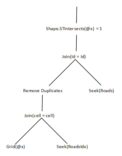
Remeber we're using SQL only as an indication of what's going on under the covers. Another way of looking at this query is:
SELECT Name
FROM
(
SELECT DISTINCT id
FROM Grid(@x) g1 JOIN RoadsIdx g2 ON g1.cell = g2.cell
) as PrimaryFilter
JOIN Roads ON PrimaryFilter.id = Roads.id
WHERE Shape.STIntersects(@x) = 1
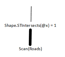
So what's really going on? These SQL queries don't really show the data flow, so let's look at a tree-like view of what's going on in the original query:
The execution proceeds by scanning the entire Roads table---this produces a large flow of data, indicated by the fat line in the tree. After our monkey business, things look a little different:
The new execution tree is much more complex, but assuming that the index is reasonably selective, no operations produce much data: gridding the parameter should be fast and produce relatively few rows, and the tables are never scanned. Despite the additional complexity, this can drastically speed up the query.
There are a number of problems with a simple grid index. Our example only has 16 cells, but this is going to be rather skimpy if we want to cover a large area and get good selectivity. If we have a much finer grid, then the number of cells---and the number of rows in our internal table---is going to get very large for large objects.
Now that we have these basics out of the way, next time we'll start talking about how SQL Server indexing actually works.
Cheers,
-Isaac
Comments
Anonymous
January 05, 2008
Looking forward to the next part Isaac, hope you had a good Christmas break. John.Anonymous
February 05, 2008
Hi Folks, Well, I never did complete my series of posts describing our indexing scheme. I guess I oughtAnonymous
February 05, 2008
Hi Folks, Well, I never did complete my series of posts describing our indexing scheme. I guess I oughtAnonymous
May 28, 2009
Hi Folks, This post contains no new information; it’s just a rollup of links to spatial indexing posts


