Excelling at Excel - Hidden cells and subtotals

When you're working in complex Excel workbooks, you may feel like you're getting lost in the clutter. There is a way to hide what you don't need to see so you can focus on the data you're really working with.

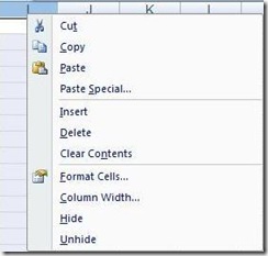
To hide a column or row, right-click its letter or number and select Hide from the dropdown menu:

You can select multiples columns and rows at once; hold the Control key if you want to select any that are non-consecutive (Columns H and M plus Row 32, for instance). Restore hidden columns and rows by selecting the columns or rows around the missing ones, then right-click and choose Unhide.

Normally, hiding rows won't interfere with any formulas so your results will remain the same even if values are called from hidden cells. But say you WANT to exclude hidden cells from a sum. Use the subtotal function with function number 109 to add up only the visible cells, as in this example:

=SUBTOTAL(109,A1:A64)

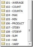
If you check the function numbers for Subtotal (viewable using auto complete when you start typing the formula into a cell), all function numbers above 100 will limit the function to visible cells only:

It's a handy trick to pull out whenever you hide cells for a reason: not just to get them out of your way, but to exclude them.

Suzanne

Comments

• Anonymous
  July 03, 2013
  thank you very much! Very useful :)

• Anonymous
  July 18, 2013
  great tip, saved me a ton of time. thanks

• Anonymous
  October 02, 2013
  The comment has been removed