Excelling at Excel: An introduction to conditional formatting

If you're new to conditional formatting in Excel, it's basically just what it sounds like: cell and text formatting that occurs when certain conditions are met. It can be used to add emphasis to your data based on whether it crosses certain thresholds that you designate.

A great example of this is a profit and loss spreadsheet: You can highlight cells with numbers in green or red to show whether they represent money made or lost.

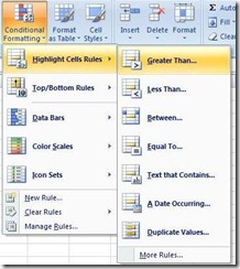
Making this magic happen is easier than you'd think! Simply select the range of cells you want to affect and click the Conditional Formatting button in the Styles section of your Home tab. In the dropdown menu, select Highlight Cell Rules and then Greater Than.

Since any Net Income above zero is profit, enter 0 in the Format cells that are GREATER THAN field and pick Green Fill with Dark Green Text from the dropdown (or Custom Format if you want to define your own). Then do the same thing for Less Than, entering 0 again and Light Red Fill with Dark Red Text. That's really all there is to it.

Explore this feature and you'll find a huge range of applications; we'll share some more helpful examples as we run into them.

Suzanne